Part I
Chapter 1 – The Best Optimizer Is between Your Ears
The Human Element of Code Optimization
This book is devoted to a topic near and dear to my heart: writing software that pushes PCs to the limit. Given run-of-the-mill software, PCs run like the 97-pound-weakling minicomputers they are. Give them the proper care, however, and those ugly boxes are capable of miracles. The key is this: Only on microcomputers do you have the run of the whole machine, without layers of operating systems, drivers, and the like getting in the way. You can do anything you want, and you can understand everything that’s going on, if you so wish.
As we’ll see shortly, you should indeed so wish.
Is performance still an issue in this era of cheap 486 computers and super-fast Pentium computers? You bet. How many programs that you use really run so fast that you wouldn’t be happier if they ran faster? We’re so used to slow software that when a compile-and-link sequence that took two minutes on a PC takes just ten seconds on a 486 computer, we’re ecstatic—when in truth we should be settling for nothing less than instantaneous response.
Impossible, you say? Not with the proper design, including incremental compilation and linking, use of extended and/or expanded memory, and well-crafted code. PCs can do just about anything you can imagine (with a few obvious exceptions, such as applications involving super-computer-class number-crunching) if you believe that it can be done, if you understand the computer inside and out, and if you’re willing to think past the obvious solution to unconventional but potentially more fruitful approaches.
My point is simply this: PCs can work wonders. It’s not easy coaxing them into doing that, but it’s rewarding—and it’s sure as heck fun. In this book, we’re going to work some of those wonders, starting…
…now.
Understanding High Performance
Before we can create high-performance code, we must understand what high performance is. The objective (not always attained) in creating high-performance software is to make the software able to carry out its appointed tasks so rapidly that it responds instantaneously, as far as the user is concerned. In other words, high-performance code should ideally run so fast that any further improvement in the code would be pointless.
Notice that the above definition most emphatically does not say anything about making the software as fast as possible. It also does not say anything about using assembly language, or an optimizing compiler, or, for that matter, a compiler at all. It also doesn’t say anything about how the code was designed and written. What it does say is that high-performance code shouldn’t get in the user’s way—and that’s all.
That’s an important distinction, because all too many programmers think that assembly language, or the right compiler, or a particular high-level language, or a certain design approach is the answer to creating high-performance code. They’re not, any more than choosing a certain set of tools is the key to building a house. You do indeed need tools to build a house, but any of many sets of tools will do. You also need a blueprint, an understanding of everything that goes into a house, and the ability to use the tools.
Likewise, high-performance programming requires a clear understanding of the purpose of the software being built, an overall program design, algorithms for implementing particular tasks, an understanding of what the computer can do and of what all relevant software is doing—and solid programming skills, preferably using an optimizing compiler or assembly language. The optimization at the end is just the finishing touch, however.
Without good design, good algorithms, and complete understanding of the program’s operation, your carefully optimized code will amount to one of mankind’s least fruitful creations—a fast slow program.
“What’s a fast slow program?” you ask. That’s a good question, and a brief (true) story is perhaps the best answer.
When Fast Isn’t Fast
In the early 1970s, as the first hand-held calculators were hitting the market, I knew a fellow named Irwin. He was a good student, and was planning to be an engineer. Being an engineer back then meant knowing how to use a slide rule, and Irwin could jockey a slipstick with the best of them. In fact, he was so good that he challenged a fellow with a calculator to a duel—and won, becoming a local legend in the process.
When you get right down to it, though, Irwin was spitting into the wind. In a few short years his hard-earned slipstick skills would be worthless, and the entire discipline would be essentially wiped from the face of the earth. What’s more, anyone with half a brain could see that changeover coming. Irwin had basically wasted the considerable effort and time he had spent optimizing his soon-to-be-obsolete skills.
What does all this have to do with programming? Plenty. When you spend time optimizing poorly-designed assembly code, or when you count on an optimizing compiler to make your code fast, you’re wasting the optimization, much as Irwin did. Particularly in assembly, you’ll find that without proper up-front design and everything else that goes into high-performance design, you’ll waste considerable effort and time on making an inherently slow program as fast as possible—which is still slow—when you could easily have improved performance a great deal more with just a little thought. As we’ll see, handcrafted assembly language and optimizing compilers matter, but less than you might think, in the grand scheme of things—and they scarcely matter at all unless they’re used in the context of a good design and a thorough understanding of both the task at hand and the PC.
Rules for Building High-Performance Code
We’ve got the following rules for creating high-performance software:
- Know where you’re going (understand the objective of the software).
- Make a big map (have an overall program design firmly in mind, so the various parts of the program and the data structures work well together).
- Make lots of little maps (design an algorithm for each separate part of the overall design).
- Know the territory (understand exactly how the computer carries out each task).
- Know when it matters (identify the portions of your programs where performance matters, and don’t waste your time optimizing the rest).
- Always consider the alternatives (don’t get stuck on a single approach; odds are there’s a better way, if you’re clever and inventive enough).
- Know how to turn on the juice (optimize the code as best you know how when it does matter).
Making rules is easy; the hard part is figuring out how to apply them in the real world. For my money, examining some actual working code is always a good way to get a handle on programming concepts, so let’s look at some of the performance rules in action.
Know Where You’re Going
If we’re going to create high-performance code, first we have to know what that code is going to do. As an example, let’s write a program that generates a 16-bit checksum of the bytes in a file. In other words, the program will add each byte in a specified file in turn into a 16-bit value. This checksum value might be used to make sure that a file hasn’t been corrupted, as might occur during transmission over a modem or if a Trojan horse virus rears its ugly head. We’re not going to do anything with the checksum value other than print it out, however; right now we’re only interested in generating that checksum value as rapidly as possible.
Make a Big Map
How are we going to generate a checksum value for a specified file? The logical approach is to get the file name, open the file, read the bytes out of the file, add them together, and print the result. Most of those actions are straightforward; the only tricky part lies in reading the bytes and adding them together.
Make Lots of Little Maps
Actually, we’re only going to make one little map, because we only have one program section that requires much thought—the section that reads the bytes and adds them up. What’s the best way to do this?
It would be convenient to load the entire file into memory and then sum the bytes in one loop. Unfortunately, there’s no guarantee that any particular file will fit in the available memory; in fact, it’s a sure thing that many files won’t fit into memory, so that approach is out.
Well, if the whole file won’t fit into memory, one byte surely will. If we read the file one byte at a time, adding each byte to the checksum value before reading the next byte, we’ll minimize memory requirements and be able to handle any size file at all.
Sounds good, eh? Listing 1.1 shows an implementation of this
approach. Listing 1.1 uses C’s read() function to read a
single byte, adds the byte into the checksum value, and loops back to
handle the next byte until the end of the file is reached. The code is
compact, easy to write, and functions perfectly—with one slight
hitch:
It’s slow.
LISTING 1.1 L1-1.C
/*
* Program to calculate the 16-bit checksum of all bytes in the
* specified file. Obtains the bytes one at a time via read(),
* letting DOS perform all data buffering.
*/
#include <stdio.h>
#include <fcntl.h>
main(int argc, char *argv[]) {
int Handle;
unsigned char Byte;
unsigned int Checksum;
int ReadLength;
if ( argc != 2 ) {
printf("usage: checksum filename\n");
exit(1);
}
if ( (Handle = open(argv[1], O_RDONLY | O_BINARY)) == -1 ) {
printf("Can't open file: %s\n", argv[1]);
exit(1);
}
/* Initialize the checksum accumulator */
Checksum = 0;
/* Add each byte in turn into the checksum accumulator */
while ( (ReadLength = read(Handle, &Byte, sizeof(Byte))) > 0 ) {
Checksum += (unsigned int) Byte;
}
if ( ReadLength == -1 ) {
printf("Error reading file %s\n", argv[1]);
exit(1);
}
/* Report the result */
printf("The checksum is: %u\n", Checksum);
exit(0);
}Table 1.1 shows the time taken for Listing 1.1 to generate a checksum of the WordPerfect version 4.2 thesaurus file, TH.WP (362,293 bytes in size), on a 10 MHz AT machine of no special parentage. Execution times are given for Listing 1.1 compiled with Borland and Microsoft compilers, with optimization both on and off; all four times are pretty much the same, however, and all are much too slow to be acceptable. Listing 1.1 requires over two and one-half minutes to checksum one file!
These results make it clear that it’s folly to rely on your compiler’s optimization to make your programs fast. Listing 1.1 is simply poorly designed, and no amount of compiler optimization will compensate for that failing. To drive home the point, Listings 1.2 and 1.3, which together are equivalent to Listing 1.1 except that the entire checksum loop is written in tight assembly code. The assembly language implementation is indeed faster than any of the C versions, as shown in Table 1.1, but it’s less than 10 percent faster, and it’s still unacceptably slow.
| Listing | Borland | Microsoft | Borland | Microsoft | Assembly | Optimization Ratio |
|---|---|---|---|---|---|---|
| (no opt) | (no opt) | (opt) | (opt) | |||
| 1 | 166.9 | 166.8 | 167.0 | 165.8 | 155.1 | 1.08 |
| 4 | 13.5 | 13.6 | 13.5 | 13.5 | … | 1.01 |
| 5 | 4.7 | 5.5 | 3.8 | 3.4 | 2.7 | 2.04 |
| Ratio best designed to worst designed | 35.51 | 30.33 | 43.95 | 48.76 | 57.44 |
Note: The execution times (in seconds) for this chapter’s listings were timed when the compiled listings were run on the WordPerfect 4.2 thesaurus file TH.WP (362,293 bytes in size), as compiled in the small model with Borland and Microsoft compilers with optimization on (opt) and off (no opt). All times were measured with Paradigm Systems’ TIMER program on a 10 MHz 1-wait-state AT clone with a 28-ms hard disk, with disk caching turned off.
LISTING 1.2 L1-2.C
/*
* Program to calculate the 16-bit checksum of the stream of bytes
* from the specified file. Obtains the bytes one at a time in
* assembler, via direct calls to DOS.
*/
#include <stdio.h>
#include <fcntl.h>
main(int argc, char *argv[]) {
int Handle;
unsigned char Byte;
unsigned int Checksum;
int ReadLength;
if ( argc != 2 ) {
printf("usage: checksum filename\n");
exit(1);
}
if ( (Handle = open(argv[1], O_RDONLY | O_BINARY)) == -1 ) {
printf("Can't open file: %s\n", argv[1]);
exit(1);
}
if ( !ChecksumFile(Handle, &Checksum) ) {
printf("Error reading file %s\n", argv[1]);
exit(1);
}
/* Report the result */
printf("The checksum is: %u\n", Checksum);
exit(0);
}LISTING 1.3 L1-3.ASM
; Assembler subroutine to perform a 16-bit checksum on the file
; opened on the passed-in handle. Stores the result in the
; passed-in checksum variable. Returns 1 for success, 0 for error.
;
; Call as:
; int ChecksumFile(unsigned int Handle, unsigned int *Checksum);
;
; where:
; Handle = handle # under which file to checksum is open
; Checksum = pointer to unsigned int variable checksum is
; to be stored in
;
; Parameter structure:
;
Parms struc
dw ? ;pushed BP
dw ? ;return address
Handle dw ?
Checksum dw ?
Parms ends
;
.model small
.data
TempWord label word
TempByte db ? ;each byte read by DOS will be stored here
db 0 ;high byte of TempWord is always 0
;for 16-bit adds
;
.code
public _ChecksumFile
_ChecksumFile proc near
push bp
mov bp,sp
push si ;save C's register variable
;
mov bx,[bp+Handle] ;get file handle
sub si,si ;zero the checksum ;accumulator
mov cx,1 ;request one byte on each ;read
mov dx,offset TempByte ;point DX to the byte in
;which DOS should store
;each byte read
ChecksumLoop:
mov ah,3fh ;DOS read file function #
int 21h ;read the byte
jc ErrorEnd ;an error occurred
and ax,ax ;any bytes read?
jz Success ;no-end of file reached-we're done
add si,[TempWord] ;add the byte into the
;checksum total
jmp ChecksumLoop
ErrorEnd:
sub ax,ax ;error
jmp short Done
Success:
mov bx,[bp+Checksum] ;point to the checksum variable
mov [bx],si ;save the new checksum
mov ax,1 ;success
;
Done:
pop si ;restore C's register variable
pop bp
ret
_ChecksumFile endp
endThe lesson is clear: Optimization makes code faster, but without proper design, optimization just creates fast slow code.
Well, then, how are we going to improve our design? Before we can do that, we have to understand what’s wrong with the current design.
Know the Territory
Just why is Listing 1.1 so slow? In a word: overhead. The C library
implements the read() function by calling DOS to read the
desired number of bytes. (I figured this out by watching the code
execute with a debugger, but you can buy library source code from both
Microsoft and Borland.) That means that Listing 1.1 (and Listing 1.3 as
well) executes one DOS function per byte processed—and DOS functions,
especially this one, come with a lot of overhead.
For starters, DOS functions are invoked with interrupts, and
interrupts are among the slowest instructions of the x86 family CPUs.
Then, DOS has to set up internally and branch to the desired function,
expending more cycles in the process. Finally, DOS has to search its own
buffers to see if the desired byte has already been read, read it from
the disk if not, store the byte in the specified location, and return.
All of that takes a long time—far, far longer than the rest of
the main loop in Listing 1.1. In short, Listing 1.1 spends virtually all
of its time executing read(), and most of that time is
spent somewhere down in DOS.
You can verify this for yourself by watching the code with a debugger or using a code profiler, but take my word for it: There’s a great deal of overhead to DOS calls, and that’s what’s draining the life out of Listing 1.1.
How can we speed up Listing 1.1? It should be clear that we must somehow avoid invoking DOS for every byte in the file, and that means reading more than one byte at a time, then buffering the data and parceling it out for examination one byte at a time. By gosh, that’s a description of C’s stream I/O feature, whereby C reads files in chunks and buffers the bytes internally, doling them out to the application as needed by reading them from memory rather than calling DOS. Let’s try using stream I/O and see what happens.
Listing 1.4 is similar to Listing 1.1, but uses fopen()
and getc() (rather than open() and
read()) to access the file being checksummed. The results
confirm our theories splendidly, and validate our new design. As shown
in Table 1.1, Listing 1.4 runs more than an order of magnitude faster
than even the assembly version of Listing 1.1, even though Listing
1.1 and Listing 1.4 look almost the same. To the casual observer,
read() and getc() would seem slightly
different but pretty much interchangeable, and yet in this application
the performance difference between the two is about the same as that
between a 4.77 MHz PC and a 16 MHz 386.
In this case that means knowing how DOS and the C/C++ file-access libraries do their work. In other words, know the territory!
LISTING 1.4 L1-4.C
/*
* Program to calculate the 16-bit checksum of the stream of bytes
* from the specified file. Obtains the bytes one at a time via
* getc(), allowing C to perform data buffering.
*/
#include <stdio.h>
main(int argc, char *argv[]) {
FILE *CheckFile;
int Byte;
unsigned int Checksum;
if ( argc != 2 ) {
printf("usage: checksum filename\n");
exit(1);
}
if ( (CheckFile = fopen(argv[1], "rb")) == NULL ) {
printf("Can't open file: %s\n", argv[1]);
exit(1);
}
/* Initialize the checksum accumulator */
Checksum = 0;
/* Add each byte in turn into the checksum accumulator */
while ( (Byte = getc(CheckFile)) != EOF ) {
Checksum += (unsigned int) Byte;
}
/* Report the result */
printf("The checksum is: %u\n", Checksum);
exit(0);
}Know When It Matters
The last section contained a particularly interesting phrase: the time-critical portions of your code. Time-critical portions of your code are those portions in which the speed of the code makes a significant difference in the overall performance of your program—and by “significant,” I don’t mean that it makes the code 100 percent faster, or 200 percent, or any particular amount at all, but rather that it makes the program more responsive and/or usable from the user’s perspective.
Don’t waste time optimizing non-time-critical code: set-up code, initialization code, and the like. Spend your time improving the performance of the code inside heavily-used loops and in the portions of your programs that directly affect response time. Notice, for example, that I haven’t bothered to implement a version of the checksum program entirely in assembly; Listings 1.2 and 1.6 call assembly subroutines that handle the time-critical operations, but C is still used for checking command-line parameters, opening files, printing, and the like.
Besides, we don’t want to optimize until the design is refined to our satisfaction, and that won’t be the case until we’ve thought about other approaches.
Always Consider the Alternatives
Listing 1.4 is good, but let’s see if there are other—perhaps less
obvious—ways to get the same results faster. Let’s start by considering
why Listing 1.4 is so much better than Listing 1.1. Like
read(), getc() calls DOS to read from the
file; the speed improvement of Listing 1.4 over Listing 1.1 occurs
because getc() reads many bytes at once via DOS, then
manages those bytes for us. That’s faster than reading them one at a
time using read()—but there’s no reason to think that it’s
faster than having our program read and manage blocks itself. Easier,
yes, but not faster.
Consider this: Every invocation of getc() involves
pushing a parameter, executing a call to the C library function, getting
the parameter (in the C library code), looking up information about the
desired stream, unbuffering the next byte from the stream, and returning
to the calling code. That takes a considerable amount of time,
especially by contrast with simply maintaining a pointer to a buffer and
whizzing through the data in the buffer inside a single loop.
There are four reasons that many programmers would give for not trying to improve on Listing 1.4:
The code is already fast enough.
The code works, and some people are content with code that works, even when it’s slow enough to be annoying.
The C library is written in optimized assembly, and it’s likely to be faster than any code that the average programmer could write to perform essentially the same function.
The C library conveniently handles the buffering of file data, and it would be a nuisance to have to implement that capability.
I’ll ignore the first reason, both because performance is no longer an issue if the code is fast enough and because the current application does not run fast enough—13 seconds is a long time. (Stop and wait for 13 seconds while you’re doing something intense, and you’ll see just how long it is.)
The second reason is the hallmark of the mediocre programmer. Know when optimization matters—and then optimize when it does!
The third reason is often fallacious. C library functions are not always written in assembly, nor are they always particularly well-optimized. (In fact, they’re often written for portability, which has nothing to do with optimization.) What’s more, they’re general-purpose functions, and often can be outperformed by well-but-not-brilliantly-written code that is well-matched to a specific task. As an example, consider Listing 1.5, which uses internal buffering to handle blocks of bytes at a time. Table 1.1 shows that Listing 1.5 is 2.5 to 4 times faster than Listing 1.4 (and as much as 49 times faster than Listing 1.1!), even though it uses no assembly at all.
LISTING 1.5 L1-5.C
/*
* Program to calculate the 16-bit checksum of the stream of bytes
* from the specified file. Buffers the bytes internally, rather
* than letting C or DOS do the work.
*/
#include <stdio.h>
#include <fcntl.h>
#include <alloc.h> /* alloc.h for Borland,
malloc.h for Microsoft */
#define BUFFER_SIZE 0x8000 /* 32Kb data buffer */
main(int argc, char *argv[]) {
int Handle;
unsigned int Checksum;
unsigned char *WorkingBuffer, *WorkingPtr;
int WorkingLength, LengthCount;
if ( argc != 2 ) {
printf("usage: checksum filename\n");
exit(1);
}
if ( (Handle = open(argv[1], O_RDONLY | O_BINARY)) == -1 ) {
printf("Can't open file: %s\n", argv[1]);
exit(1);
}
/* Get memory in which to buffer the data */
if ( (WorkingBuffer = malloc(BUFFER_SIZE)) == NULL ) {
printf("Can't get enough memory\n");
exit(1);
}
/* Initialize the checksum accumulator */
Checksum = 0;
/* Process the file in BUFFER_SIZE chunks */
do {
if ( (WorkingLength = read(Handle, WorkingBuffer,
BUFFER_SIZE)) == -1 ) {
printf("Error reading file %s\n", argv[1]);
exit(1);
}
/* Checksum this chunk */
WorkingPtr = WorkingBuffer;
LengthCount = WorkingLength;
while ( LengthCount-- ) {
/* Add each byte in turn into the checksum accumulator */
Checksum += (unsigned int) *WorkingPtr++;
}
} while ( WorkingLength );
/* Report the result */
printf("The checksum is: %u\n", Checksum);
exit(0);
}That brings us to the fourth reason: avoiding an internal-buffered implementation like Listing 1.5 because of the difficulty of coding such an approach. True, it is easier to let a C library function do the work, but it’s not all that hard to do the buffering internally. The key is the concept of handling data in restartable blocks; that is, reading a chunk of data, operating on the data until it runs out, suspending the operation while more data is read in, and then continuing as though nothing had happened.
In Listing 1.5 the restartable block implementation is pretty simple because checksumming works with one byte at a time, forgetting about each byte immediately after adding it into the total. Listing 1.5 reads in a block of bytes from the file, checksums the bytes in the block, and gets another block, repeating the process until the entire file has been processed. In Chapter 5, we’ll see a more complex restartable block implementation, involving searching for text strings.
At any rate, Listing 1.5 isn’t much more complicated than Listing 1.4—and it’s a lot faster. Always consider the alternatives; a bit of clever thinking and program redesign can go a long way.
Know How to Turn On the Juice
I have said time and again that optimization is pointless until the design is settled. When that time comes, however, optimization can indeed make a significant difference. Table 1.1 indicates that the optimized version of Listing 1.5 produced by Microsoft C outperforms an unoptimized version of the same code by more than 60 percent. What’s more, a mostly-assembly version of Listing 1.5, shown in Listings 1.6 and 1.7, outperforms even the best-optimized C version of Listing 1.5 by 26 percent. These are considerable improvements, well worth pursuing—once the design has been maxed out.
LISTING 1.6 L1-6.C
/*
* Program to calculate the 16-bit checksum of the stream of bytes
* from the specified file. Buffers the bytes internally, rather
* than letting C or DOS do the work, with the time-critical
* portion of the code written in optimized assembler.
*/
#include <stdio.h>
#include <fcntl.h>
#include <alloc.h> /* alloc.h for Borland,
malloc.h for Microsoft */
#define BUFFER_SIZE 0x8000 /* 32K data buffer */
main(int argc, char *argv[]) {
int Handle;
unsigned int Checksum;
unsigned char *WorkingBuffer;
int WorkingLength;
if ( argc != 2 ) {
printf("usage: checksum filename\n");
exit(1);
}
if ( (Handle = open(argv[1], O_RDONLY | O_BINARY)) == -1 ) {
printf("Can't open file: %s\n", argv[1]);
exit(1);
}
/* Get memory in which to buffer the data */
if ( (WorkingBuffer = malloc(BUFFER_SIZE)) == NULL ) {
printf("Can't get enough memory\n");
exit(1);
}
/* Initialize the checksum accumulator */
Checksum = 0;
/* Process the file in 32K chunks */
do {
if ( (WorkingLength = read(Handle, WorkingBuffer,
BUFFER_SIZE)) == -1 ) {
printf("Error reading file %s\n", argv[1]);
exit(1);
}
/* Checksum this chunk if there's anything in it */
if ( WorkingLength )
ChecksumChunk(WorkingBuffer, WorkingLength, &Checksum);
} while ( WorkingLength );
/* Report the result */
printf("The checksum is: %u\n", Checksum);
exit(0);
}LISTING 1.7 L1-7.ASM
; Assembler subroutine to perform a 16-bit checksum on a block of
; bytes 1 to 64K in size. Adds checksum for block into passed-in
; checksum.
;
; Call as:
; void ChecksumChunk(unsigned char *Buffer,
; unsigned int BufferLength, unsigned int *Checksum);
;
; where:
; Buffer = pointer to start of block of bytes to checksum
; BufferLength = # of bytes to checksum (0 means 64K, not 0)
; Checksum = pointer to unsigned int variable checksum is
;stored in
;
; Parameter structure:
;
Parms struc
dw ? ;pushed BP
dw ? ;return address
Buffer dw ?
BufferLength dw ?
Checksum dw ?
Parms ends
;
.model small
.code
public _ChecksumChunk
_ChecksumChunk proc near
push bp
mov bp,sp
push si ;save C's register variable
;
cld ;make LODSB increment SI
mov si,[bp+Buffer] ;point to buffer
mov cx,[bp+BufferLength] ;get buffer length
mov bx,[bp+Checksum] ;point to checksum variable
mov dx,[bx] ;get the current checksum
sub ah,ah ;so AX will be a 16-bit value after LODSB
ChecksumLoop:
lodsb ;get the next byte
add dx,ax ;add it into the checksum total
loop ChecksumLoop ;continue for all bytes in block
mov [bx],dx ;save the new checksum
;
pop si ;restore C's register variable
pop bp
ret
_ChecksumChunk endp
endNote that in Table 1.1, optimization makes little difference except in the case of Listing 1.5, where the design has been refined considerably. Execution time in the other cases is dominated by time spent in DOS and/or the C library, so optimization of the code you write is pretty much irrelevant. What’s more, while the approximately two-times improvement we got by optimizing is not to be sneezed at, it pales against the up-to-50-times improvement we got by redesigning.
By the way, the execution times even of Listings 1.6 and 1.7 are dominated by DOS disk access times. If a disk cache is enabled and the file to be checksummed is already in the cache, the assembly version is three times as fast as the C version. In other words, the inherent nature of this application limits the performance improvement that can be obtained via assembly. In applications that are more CPU-intensive and less disk-bound, particularly those applications in which string instructions and/or unrolled loops can be used effectively, assembly tends to be considerably faster relative to C than it is in this very specific case.
All this is basically a way of saying: Know where you’re going, know the territory, and know when it matters.
Where We’ve Been, What We’ve Seen
What have we learned? Don’t let other people’s code—even DOS—do the work for you when speed matters, at least not without knowing what that code does and how well it performs.
Optimization only matters after you’ve done your part on the program design end. Consider the ratios on the vertical axis of Table 1.1, which show that optimization is almost totally wasted in the checksumming application without an efficient design. Optimization is no panacea. Table 1.1 shows a two-times improvement from optimization—and a 50-times-plus improvement from redesign. The longstanding debate about which C compiler optimizes code best doesn’t matter quite so much in light of Table 1.1, does it? Your organic optimizer matters much more than your compiler’s optimizer, and there’s always assembly for those usually small sections of code where performance really matters.
Where We’re Going
This chapter has presented a quick step-by-step overview of the design process. I’m not claiming that this is the only way to create high-performance code; it’s just an approach that works for me. Create code however you want, but never forget that design matters more than detailed optimization. Never stop looking for inventive ways to boost performance—and never waste time speeding up code that doesn’t need to be sped up.
I’m going to focus on specific ways to create high-performance code from now on. In Chapter 5, we’ll continue to look at restartable blocks and internal buffering, in the form of a program that searches files for text strings.
Chapter 2 – A World Apart
The Unique Nature of Assembly Language Optimization
As I showed in the previous chapter, optimization is by no means always a matter of “dropping into assembly.” In fact, in performance tuning high-level language code, assembly should be used rarely, and then only after you’ve made sure a badly chosen or clumsily implemented algorithm isn’t eating you alive. Certainly if you use assembly at all, make absolutely sure you use it right. The potential of assembly code to run slowly is poorly understood by a lot of people, but that potential is great, especially in the hands of the ignorant.
Truly great optimization, however, happens only at the assembly level, and it happens in response to a set of dynamics that is totally different from that governing C/C++ or Pascal optimization. I’ll be speaking of assembly-level optimization time and again in this book, but when I do, I think it will be helpful if you have a grasp of those assembly specific dynamics.
As usual, the best way to wade in is to present a real-world example.
Instructions: The Individual versus the Collective
Some time ago, I was asked to work over a critical assembly subroutine in order to make it run as fast as possible. The task of the subroutine was to construct a nibble out of four bits read from different bytes, rotating and combining the bits so that they ultimately ended up neatly aligned in bits 3-0 of a single byte. (In case you’re curious, the object was to construct a 16-color pixel from bits scattered over 4 bytes.) I examined the subroutine line by line, saving a cycle here and a cycle there, until the code truly seemed to be optimized. When I was done, the key part of the code looked something like this:
LoopTop:
lodsb ;get the next byte to extract a bit from
and al,ah ;isolate the bit we want
rol al,cl ;rotate the bit into the desired position
or bl,al ;insert the bit into the final nibble
dec cx ;the next bit goes 1 place to the right
dec dx ;count down the number of bits
jnz LoopTop ;process the next bit, if anyNow, it’s hard to write code that’s much faster than seven instructions, only one of which accesses memory, and most programmers would have called it a day at this point. Still, something bothered me, so I spent a bit of time going over the code again. Suddenly, the answer struck me—the code was rotating each bit into place separately, so that a multibit rotation was being performed every time through the loop, for a total of four separate time-consuming multibit rotations!
I changed the code to the following:
LoopTop:
lodsb ;get the next byte to extract a bit from
and al,ah ;isolate the bit we want
or bl,al ;insert the bit into the final nibble
rol bl,1 ;make room for the next bit
dec dx ;count down the number of bits
jnz LoopTop ;process the next bit, if any
rol bl,cl ;rotate all four bits into their final
; positions at the same timeThis moved the costly multibit rotation out of the loop so that it
was performed just once, rather than four times. While the code may not
look much different from the original, and in fact still contains
exactly the same number of instructions, the performance of the entire
subroutine improved by about 10 percent from just this one change.
(Incidentally, that wasn’t the end of the optimization; I eliminated the
DEC and JNZ instructions by expanding the four
iterations of the loop—but that’s a tale for another chapter.)
The point is this: To write truly superior assembly programs, you need to know what the various instructions do and which instructions execute fastest…and more. You must also learn to look at your programming problems from a variety of perspectives so that you can put those fast instructions to work in the most effective ways.
Assembly Is Fundamentally Different
Is it really so hard as all that to write good assembly code for the PC? Yes! Thanks to the decidedly quirky nature of the x86 family CPUs, assembly language differs fundamentally from other languages, and is undeniably harder to work with. On the other hand, the potential of assembly code is much greater than that of other languages, as well.
To understand why this is so, consider how a program gets written. A programmer examines the requirements of an application, designs a solution at some level of abstraction, and then makes that design come alive in a code implementation. If not handled properly, the transformation that takes place between conception and implementation can reduce performance tremendously; for example, a programmer who implements a routine to search a list of 100,000 sorted items with a linear rather than binary search will end up with a disappointingly slow program.
Transformation Inefficiencies
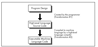
No matter how well an implementation is derived from the corresponding design, however, high-level languages like C/C++ and Pascal inevitably introduce additional transformation inefficiencies, as shown in Figure 2.1.
The process of turning a design into executable code by way of a high-level language involves two transformations: one performed by the programmer to generate source code, and another performed by the compiler to turn source code into machine language instructions. Consequently, the machine language code generated by compilers is usually less than optimal given the requirements of the original design.
High-level languages provide artificial environments that lend themselves relatively well to human programming skills, in order to ease the transition from design to implementation. The price for this ease of implementation is a considerable loss of efficiency in transforming source code into machine language. This is particularly true given that the x86 family in real and 16-bit protected mode, with its specialized memory-addressing instructions and segmented memory architecture, does not lend itself particularly well to compiler design. Even the 32-bit mode of the 386 and its successors, with their more powerful addressing modes, offer fewer registers than compilers would like.
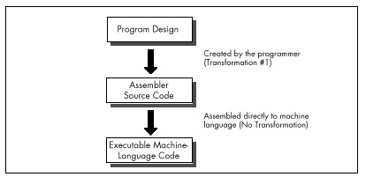
Assembly, on the other hand, is simply a human-oriented representation of machine language. As a result, assembly provides a difficult programming environment—the bare hardware and systems software of the computer—but properly constructed assembly programs suffer no transformation loss, as shown in Figure 2.2.
Only one transformation is required when creating an assembler program, and that single transformation is completely under the programmer’s control. Assemblers perform no transformation from source code to machine language; instead, they merely map assembler instructions to machine language instructions on a one-to-one basis. As a result, the programmer is able to produce machine language code that’s precisely tailored to the needs of each task a given application requires.
The key, of course, is the programmer, since in assembly the programmer must essentially perform the transformation from the application specification to machine language entirely on his or her own. (The assembler merely handles the direct translation from assembly to machine language.)
Self-Reliance
The first part of assembly language optimization, then, is self. An assembler is nothing more than a tool to let you design machine-language programs without having to think in hexadecimal codes. So assembly language programmers—unlike all other programmers—must take full responsibility for the quality of their code. Since assemblers provide little help at any level higher than the generation of machine language, the assembly programmer must be capable both of coding any programming construct directly and of controlling the PC at the lowest practical level—the operating system, the BIOS, even the hardware where necessary. High-level languages handle most of this transparently to the programmer, but in assembly everything is fair—and necessary—game, which brings us to another aspect of assembly optimization: knowledge.
Knowledge
In the PC world, you can never have enough knowledge, and every item you add to your store will make your programs better. Thorough familiarity with both the operating system APIs and BIOS interfaces is important; since those interfaces are well-documented and reasonably straightforward, my advice is to get a good book or two and bring yourself up to speed. Similarly, familiarity with the PC hardware is required. While that topic covers a lot of ground—display adapters, keyboards, serial ports, printer ports, timer and DMA channels, memory organization, and more—most of the hardware is well-documented, and articles about programming major hardware components appear frequently in the literature, so this sort of knowledge can be acquired readily enough.
The single most critical aspect of the hardware, and the one about which it is hardest to learn, is the CPU. The x86 family CPUs have a complex, irregular instruction set, and, unlike most processors, they are neither straightforward nor well-documented true code performance. What’s more, assembly is so difficult to learn that most articles and books that present assembly code settle for code that just works, rather than code that pushes the CPU to its limits. In fact, since most articles and books are written for inexperienced assembly programmers, there is very little information of any sort available about how to generate high-quality assembly code for the x86 family CPUs. As a result, knowledge about programming them effectively is by far the hardest knowledge to gather. A good portion of this book is devoted to seeking out such knowledge.
The Flexible Mind
Is the never-ending collection of information all there is to the assembly optimization, then? Hardly. Knowledge is simply a necessary base on which to build. Let’s take a moment to examine the objectives of good assembly programming, and the remainder of the forces that act on assembly optimization will fall into place.
Basically, there are only two possible objectives to high-performance assembly programming: Given the requirements of the application, keep to a minimum either the number of processor cycles the program takes to run, or the number of bytes in the program, or some combination of both. We’ll look at ways to achieve both objectives, but we’ll more often be concerned with saving cycles than saving bytes, for the PC generally offers relatively more memory than it does processing horsepower. In fact, we’ll find that two-to-three times performance improvements over already tight assembly code are often possible if we’re willing to spend additional bytes in order to save cycles. It’s not always desirable to use such techniques to speed up code, due to the heavy memory requirements—but it is almost always possible.
You will notice that my short list of objectives for high-performance assembly programming does not include traditional objectives such as easy maintenance and speed of development. Those are indeed important considerations—to persons and companies that develop and distribute software. People who actually buy software, on the other hand, care only about how well that software performs, not how it was developed nor how it is maintained. These days, developers spend so much time focusing on such admittedly important issues as code maintainability and reusability, source code control, choice of development environment, and the like that they often forget rule #1: From the user’s perspective, performance is fundamental.
Knowledge of the sort described earlier is absolutely essential to fulfilling either of the objectives of assembly programming. What that knowledge doesn’t do by itself is meet the need to write code that both performs to the requirements of the application at hand and also operates as efficiently as possible in the PC environment. Knowledge makes that possible, but your programming instincts make it happen. And it is that intuitive, on-the-fly integration of a program specification and a sea of facts about the PC that is the heart of the Zen-class assembly optimization.
As with Zen of any sort, mastering that Zen of assembly language is more a matter of learning than of being taught. You will have to find your own path of learning, although I will start you on your way with this book. The subtle facts and examples I provide will help you gain the necessary experience, but you must continue the journey on your own. Each program you create will expand your programming horizons and increase the options available to you in meeting the next challenge. The ability of your mind to find surprising new and better ways to craft superior code from a concept—the flexible mind, if you will—is the linchpin of good assembler code, and you will develop this skill only by doing.
Never underestimate the importance of the flexible mind. Good assembly code is better than good compiled code. Many people would have you believe otherwise, but they’re wrong. That doesn’t mean that high-level languages are useless; far from it. High-level languages are the best choice for the majority of programmers, and for the bulk of the code of most applications. When the best code—the fastest or smallest code possible—is needed, though, assembly is the only way to go.
Simple logic dictates that no compiler can know as much about what a piece of code needs to do or adapt as well to those needs as the person who wrote the code. Given that superior information and adaptability, an assembly language programmer can generate better code than a compiler, all the more so given that compilers are constrained by the limitations of high-level languages and by the process of transformation from high-level to machine language. Consequently, carefully optimized assembly is not just the language of choice but the only choice for the 1 percent to 10 percent of code—usually consisting of small, well-defined subroutines—that determines overall program performance, and it is the only choice for code that must be as compact as possible, as well. In the run-of-the-mill, non-time-critical portions of your programs, it makes no sense to waste time and effort on writing optimized assembly code—concentrate your efforts on loops and the like instead; but in those areas where you need the finest code quality, accept no substitutes.
Note that I said that an assembly programmer can generate better code than a compiler, not will generate better code. While it is true that good assembly code is better than good compiled code, it is also true that bad assembly code is often much worse than bad compiled code; since the assembly programmer has so much control over the program, he or she has virtually unlimited opportunities to waste cycles and bytes. The sword cuts both ways, and good assembly code requires more, not less, forethought and planning than good code written in a high-level language.
The gist of all this is simply that good assembly programming is done in the context of a solid overall framework unique to each program, and the flexible mind is the key to creating that framework and holding it together.
Where to Begin?
To summarize, the skill of assembly language optimization is a combination of knowledge, perspective, and a way of thought that makes possible the genesis of absolutely the fastest or the smallest code. With that in mind, what should the first step be? Development of the flexible mind is an obvious step. Still, the flexible mind is no better than the knowledge at its disposal. The first step in the journey toward mastering optimization at that exalted level, then, would seem to be learning how to learn.
Chapter 3 – Assume Nothing
Understanding and Using the Zen Timer
When you’re pushing the envelope in writing optimized PC code, you’re likely to become more than a little compulsive about finding approaches that let you wring more speed from your computer. In the process, you’re bound to make mistakes, which is fine—as long as you watch for those mistakes and learn from them.
A case in point: A few years back, I came across an article about 8088 assembly language called “Optimizing for Speed.” Now, “optimize” is not a word to be used lightly; Webster’s Ninth New Collegiate Dictionary defines optimize as “to make as perfect, effective, or functional as possible,” which certainly leaves little room for error. The author had, however, chosen a small, well-defined 8088 assembly language routine to refine, consisting of about 30 instructions that did nothing more than expand 8 bits to 16 bits by duplicating each bit.
The author of “Optimizing” had clearly fine-tuned the code with care, examining alternative instruction sequences and adding up cycles until he arrived at an implementation he calculated to be nearly 50 percent faster than the original routine. In short, he had used all the information at his disposal to improve his code, and had, as a result, saved cycles by the bushel. There was, in fact, only one slight problem with the optimized version of the routine….
It ran slower than the original version!
The Costs of Ignorance
As diligent as the author had been, he had nonetheless committed a cardinal sin of x86 assembly language programming: He had assumed that the information available to him was both correct and complete. While the execution times provided by Intel for its processors are indeed correct, they are incomplete; the other—and often more important—part of code performance is instruction fetch time, a topic to which I will return in later chapters.
Had the author taken the time to measure the true performance of his code, he wouldn’t have put his reputation on the line with relatively low-performance code. What’s more, had he actually measured the performance of his code and found it to be unexpectedly slow, curiosity might well have led him to experiment further and thereby add to his store of reliable information about the CPU.
Assume nothing. I cannot emphasize this strongly enough—when you care about performance, do your best to improve the code and then measure the improvement. If you don’t measure performance, you’re just guessing, and if you’re guessing, you’re not very likely to write top-notch code.
Ignorance about true performance can be costly. When I wrote video games for a living, I spent days at a time trying to wring more performance from my graphics drivers. I rewrote whole sections of code just to save a few cycles, juggled registers, and relied heavily on blurry-fast register-to-register shifts and adds. As I was writing my last game, I discovered that the program ran perceptibly faster if I used look-up tables instead of shifts and adds for my calculations. It shouldn’t have run faster, according to my cycle counting, but it did. In truth, instruction fetching was rearing its head again, as it often does, and the fetching of the shifts and adds was taking as much as four times the nominal execution time of those instructions.
Ignorance can also be responsible for considerable wasted effort. I recall a debate in the letters column of one computer magazine about exactly how quickly text can be drawn on a Color/Graphics Adapter (CGA) screen without causing snow. The letter-writers counted every cycle in their timing loops, just as the author in the story that started this chapter had. Like that author, the letter-writers had failed to take the prefetch queue into account. In fact, they had neglected the effects of video wait states as well, so the code they discussed was actually much slower than their estimates. The proper test would, of course, have been to run the code to see if snow resulted, since the only true measure of code performance is observing it in action.
The Zen Timer
Clearly, one key to mastering Zen-class optimization is a tool with which to measure code performance. The most accurate way to measure performance is with expensive hardware, but reasonable measurements at no cost can be made with the PC’s 8253 timer chip, which counts at a rate of slightly over 1,000,000 times per second. The 8253 can be started at the beginning of a block of code of interest and stopped at the end of that code, with the resulting count indicating how long the code took to execute with an accuracy of about 1 microsecond. (A microsecond is one millionth of a second, and is abbreviated µs). To be precise, the 8253 counts once every 838.1 nanoseconds. (A nanosecond is one billionth of a second, and is abbreviated ns.)
Listing 3.1 shows 8253-based timer software, consisting of three
subroutines: ZTimerOn, ZTimerOff, and
ZTimerReport. For the remainder of this book, I’ll refer to
these routines collectively as the “Zen timer.” C-callable versions of
the two precision Zen timers are presented in Chapter K on the companion
CD-ROM.
LISTING 3.1 PZTIMER.ASM
; The precision Zen timer (PZTIMER.ASM)
;
; Uses the 8253 timer to time the performance of code that takes
; less than about 54 milliseconds to execute, with a resolution
; of better than 10 microseconds.
;
; By Michael Abrash
;
; Externally callable routines:
;
; ZTimerOn: Starts the Zen timer, with interrupts disabled.
;
; ZTimerOff: Stops the Zen timer, saves the timer count,
; times the overhead code, and restores interrupts to the
; state they were in when ZTimerOn was called.
;
; ZTimerReport: Prints the net time that passed between starting
; and stopping the timer.
;
; Note: If longer than about 54 ms passes between ZTimerOn and
; ZTimerOff calls, the timer turns over and the count is
; inaccurate. When this happens, an error message is displayed
; instead of a count. The long-period Zen timer should be used
; in such cases.
;
; Note: Interrupts *MUST* be left off between calls to ZTimerOn
; and ZTimerOff for accurate timing and for detection of
; timer overflow.
;
; Note: These routines can introduce slight inaccuracies into the
; system clock count for each code section timed even if
; timer 0 doesn't overflow. If timer 0 does overflow, the
; system clock can become slow by virtually any amount of
; time, since the system clock can't advance while the
; precison timer is timing. Consequently, it's a good idea
; to reboot at the end of each timing session. (The
; battery-backed clock, if any, is not affected by the Zen
; timer.)
;
; All registers, and all flags except the interrupt flag, are
; preserved by all routines. Interrupts are enabled and then disabled
; by ZTimerOn, and are restored by ZTimerOff to the state they were
; in when ZTimerOn was called.
;
Code segment word public 'CODE'
assume cs:Code, ds:nothing
public ZTimerOn, ZTimerOff, ZTimerReport
;
; Base address of the 8253 timer chip.
;
BASE_8253 equ 40h
;
; The address of the timer 0 count registers in the 8253.
;
TIMER_0_8253 equ BASE_8253 + 0
;
; The address of the mode register in the 8253.
;
MODE_8253 equ BASE_8253 + 3
;
; The address of Operation Command Word 3 in the 8259 Programmable
; Interrupt Controller (PIC) (write only, and writable only when
; bit 4 of the byte written to this address is 0 and bit 3 is 1).
;
OCW3 equ 20h
;
; The address of the Interrupt Request register in the 8259 PIC
; (read only, and readable only when bit 1 of OCW3 = 1 and bit 0
; of OCW3 = 0).
;
IRR equ 20h
;
; Macro to emulate a POPF instruction in order to fix the bug in some
; 80286 chips which allows interrupts to occur during a POPF even when
; interrupts remain disabled.
;
MPOPF macro
local p1, p2
jmp short p2
p1: iret ; jump to pushed address & pop flags
p2: push cs ; construct far return address to
call p1 ; the next instruction
endm
;
; Macro to delay briefly to ensure that enough time has elapsed
; between successive I/O accesses so that the device being accessed
; can respond to both accesses even on a very fast PC.
;
DELAY macro
jmp $+2
jmp $+2
jmp $+2
endm
OriginalFlags db ? ; storage for upper byte of
; FLAGS register when
; ZTimerOn called
TimedCount dw ? ; timer 0 count when the timer
; is stopped
ReferenceCount dw ? ; number of counts required to
; execute timer overhead code
OverflowFlag db ? ; used to indicate whether the
; timer overflowed during the
; timing interval
;
; String printed to report results.
;
OutputStr label byte
db 0dh, 0ah, 'Timed count: ', 5 dup (?)
ASCIICountEnd label byte
db ' microseconds', 0dh, 0ah
db '$'
;
; String printed to report timer overflow.
;
OverflowStr label byte
db 0dh, 0ah
db '****************************************************'
db 0dh, 0ah
db '* The timer overflowed, so the interval timed was *'
db 0dh, 0ah
db '* too long for the precision timer to measure. *'
db 0dh, 0ah
db '* Please perform the timing test again with the *'
db 0dh, 0ah
db '* long-period timer. *'
db 0dh, 0ah
db '****************************************************'
db 0dh, 0ah
db '$'
; ********************************************************************
; * Routine called to start timing. *
; ********************************************************************
ZTimerOn proc near
;
; Save the context of the program being timed.
;
push ax
pushf
pop ax ; get flags so we can keep
; interrupts off when leaving
; this routine
mov cs:[OriginalFlags],ah ; remember the state of the
; Interrupt flag
and ah,0fdh ; set pushed interrupt flag
; to 0
push ax
;
; Turn on interrupts, so the timer interrupt can occur if it's
; pending.
;
sti
;
; Set timer 0 of the 8253 to mode 2 (divide-by-N), to cause
; linear counting rather than count-by-two counting. Also
; leaves the 8253 waiting for the initial timer 0 count to
; be loaded.
;
mov al,00110100b ;mode 2
out MODE_8253,al
;
; Set the timer count to 0, so we know we won't get another
; timer interrupt right away.
; Note: this introduces an inaccuracy of up to 54 ms in the system
; clock count each time it is executed.
;
DELAY
sub al,al
out TIMER_0_8253,al ;lsb
DELAY
out TIMER_0_8253,al ;msb
;
; Wait before clearing interrupts to allow the interrupt generated
; when switching from mode 3 to mode 2 to be recognized. The delay
; must be at least 210 ns long to allow time for that interrupt to
; occur. Here, 10 jumps are used for the delay to ensure that the
; delay time will be more than long enough even on a very fast PC.
;
rept 10
jmp $+2
endm
;
; Disable interrupts to get an accurate count.
;
cli
;
; Set the timer count to 0 again to start the timing interval.
;
mov al,00110100b ; set up to load initial
out MODE_8253,al ; timer count
DELAY
sub al,al
out TIMER_0_8253,al ; load count lsb
DELAY
out TIMER_0_8253,al; load count msb
;
; Restore the context and return.
;
MPOPF ; keeps interrupts off
pop ax
ret
ZTimerOn endp
;********************************************************************
;* Routine called to stop timing and get count. *
;********************************************************************
ZTimerOff proc near
;
; Save the context of the program being timed.
;
push ax
push cx
pushf
;
; Latch the count.
;
mov al,00000000b ; latch timer 0
out MODE_8253,al
;
; See if the timer has overflowed by checking the 8259 for a pending
; timer interrupt.
;
mov al,00001010b ; OCW3, set up to read
out OCW3,al ; Interrupt Request register
DELAY
in al,IRR ; read Interrupt Request
; register
and al,1 ; set AL to 1 if IRQ0 (the
; timer interrupt) is pending
mov cs:[OverflowFlag],al; store the timer overflow
; status
;
; Allow interrupts to happen again.
;
sti
;
; Read out the count we latched earlier.
;
in al,TIMER_0_8253 ; least significant byte
DELAY
mov ah,al
in al,TIMER_0_8253 ; most significant byte
xchg ah,al
neg ax ; convert from countdown
; remaining to elapsed
; count
mov cs:[TimedCount],ax
; Time a zero-length code fragment, to get a reference for how
; much overhead this routine has. Time it 16 times and average it,
; for accuracy, rounding the result.
;
mov cs:[ReferenceCount],0
mov cx,16
cli ; interrupts off to allow a
; precise reference count
RefLoop:
call ReferenceZTimerOn
call ReferenceZTimerOff
loop RefLoop
sti
add cs:[ReferenceCount],8; total + (0.5 * 16)
mov cl,4
shr cs:[ReferenceCount],cl; (total) / 16 + 0.5
;
; Restore original interrupt state.
;
pop ax ; retrieve flags when called
mov ch,cs:[OriginalFlags] ; get back the original upper
; byte of the FLAGS register
and ch,not 0fdh ; only care about original
; interrupt flag...
and ah,0fdh ; ...keep all other flags in
; their current condition
or ah,ch ; make flags word with original
; interrupt flag
push ax ; prepare flags to be popped
;
; Restore the context of the program being timed and return to it.
;
MPOPF ; restore the flags with the
; original interrupt state
pop cx
pop ax
ret
ZTimerOff endp
;
; Called by ZTimerOff to start timer for overhead measurements.
;
ReferenceZTimerOn proc near
;
; Save the context of the program being timed.
;
push ax
pushf ; interrupts are already off
;
; Set timer 0 of the 8253 to mode 2 (divide-by-N), to cause
; linear counting rather than count-by-two counting.
;
mov al,00110100b ; set up to load
out MODE_8253,al ; initial timer count
DELAY
;
; Set the timer count to 0.
;
sub al,al
out TIMER_0_8253,al; load count lsb
DELAY
out TIMER_0_8253,al; load count msb
;
; Restore the context of the program being timed and return to it.
;
MPOPF
pop ax
ret
ReferenceZTimerOn endp
;
; Called by ZTimerOff to stop timer and add result to ReferenceCount
; for overhead measurements.
;
ReferenceZTimerOff proc near
;
; Save the context of the program being timed.
;
push ax
push cx
pushf
;
; Latch the count and read it.
;
mov al,00000000b ; latch timer 0
out MODE_8253,al
DELAY
in al,TIMER_0_8253 ; lsb
DELAY
mov ah,al
in al,TIMER_0_8253 ; msb
xchg ah,al
neg ax ; convert from countdown
; remaining to amount
; counted down
add cs:[ReferenceCount],ax
;
; Restore the context of the program being timed and return to it.
;
MPOPF
pop cx
pop ax
ret
ReferenceZTimerOff endp
; ********************************************************************
; * Routine called to report timing results. *
; ********************************************************************
ZTimerReport proc near
pushf
push ax
push bx
push cx
push dx
push si
push ds
;
push cs ; DOS functions require that DS point
pop ds ; to text to be displayed on the screen
assume ds :Code
;
; Check for timer 0 overflow.
;
cmp [OverflowFlag],0
jz PrintGoodCount
mov dx,offset OverflowStr
mov ah,9
int 21h
jmp short EndZTimerReport
;
; Convert net count to decimal ASCII in microseconds.
;
PrintGoodCount:
mov ax,[TimedCount]
sub ax,[ReferenceCount]
mov si,offset ASCIICountEnd - 1
;
; Convert count to microseconds by multiplying by .8381.
;
mov dx, 8381
mul dx
mov bx, 10000
div bx ;* .8381 = * 8381 / 10000
;
; Convert time in microseconds to 5 decimal ASCII digits.
;
mov bx, 10
mov cx, 5
CTSLoop:
sub dx, dx
div bx
add dl,'0'
mov [si],dl
dec si
loop CTSLoop
;
; Print the results.
;
mov ah, 9
mov dx, offset OutputStr
int 21h
;
EndZTimerReport:
pop ds
pop si
pop dx
pop cx
pop bx
pop ax
MPOPF
ret
ZTimerReport endp
Code ends
endThe Zen Timer Is a Means, Not an End
We’re going to spend the rest of this chapter seeing what the Zen timer can do, examining how it works, and learning how to use it. I’ll be using the Zen timer again and again over the course of this book, so it’s essential that you learn what the Zen timer can do and how to use it. On the other hand, it is by no means essential that you understand exactly how the Zen timer works. (Interesting, yes; essential, no.)
In other words, the Zen timer isn’t really part of the knowledge we seek; rather, it’s one tool with which we’ll acquire that knowledge. Consequently, you shouldn’t worry if you don’t fully grasp the inner workings of the Zen timer. Instead, focus on learning how to use it, and you’ll be on the right road.
Starting the Zen Timer
ZTimerOn is called at the start of a segment of code to
be timed. ZTimerOn saves the context of the calling code,
disables interrupts, sets timer 0 of the 8253 to mode 2 (divide-by-N
mode), sets the initial timer count to 0, restores the context of the
calling code, and returns. (I’d like to note that while Intel’s
documentation for the 8253 seems to indicate that a timer won’t reset to
0 until it finishes counting down, in actual practice, timers seem to
reset to 0 as soon as they’re loaded.)
Two aspects of ZTimerOn are worth discussing further.
One point of interest is that ZTimerOn disables interrupts.
(ZTimerOff later restores interrupts to the state they were
in when ZTimerOn was called.) Were interrupts not disabled
by ZTimerOn, keyboard, mouse, timer, and other interrupts
could occur during the timing interval, and the time required to service
those interrupts would incorrectly and erratically appear to be part of
the execution time of the code being measured. As a result, code timed
with the Zen timer should not expect any hardware interrupts to occur
during the interval between any call to ZTimerOn and the
corresponding call to ZTimerOff, and should not enable
interrupts during that time.
Time and the PC
A second interesting point about ZTimerOn is that it may
introduce some small inaccuracy into the system clock time whenever it
is called. To understand why this is so, we need to examine the way in
which both the 8253 and the PC’s system clock (which keeps the current
time) work.
The 8253 actually contains three timers, as shown in Figure 3.1. All three timers are driven by the system board’s 14.31818 MHz crystal, divided by 12 to yield a 1.19318 MHz clock to the timers, so the timers count once every 838.1 ns. Each of the three timers counts down in a programmable way, generating a signal on its output pin when it counts down to 0. Each timer is capable of being halted at any time via a 0 level on its gate input; when a timer’s gate input is 1, that timer counts constantly. All in all, the 8253’s timers are inherently very flexible timing devices; unfortunately, much of that flexibility depends on how the timers are connected to external circuitry, and in the PC the timers are connected with specific purposes in mind.
Timer 2 drives the speaker, although it can be used for other timing purposes when the speaker is not in use. As shown in Figure 3.1, timer 2 is the only timer with a programmable gate input in the PC; that is, timer 2 is the only timer that can be started and stopped under program control in the manner specified by Intel. On the other hand, the output of timer 2 is connected to nothing other than the speaker. In particular, timer 2 cannot generate an interrupt to get the 8088’s attention.
Timer 1 is dedicated to providing dynamic RAM refresh, and should not be tampered with lest system crashes result.
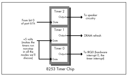
Finally, timer 0 is used to drive the system clock. As programmed by the BIOS at power-up, every 65,536 (64K) counts, or 54.925 milliseconds, timer 0 generates a rising edge on its output line. (A millisecond is one-thousandth of a second, and is abbreviated ms.) This line is connected to the hardware interrupt 0 (IRQ0) line on the system board, so every 54.925 ms, timer 0 causes hardware interrupt 0 to occur.
The interrupt vector for IRQ0 is set by the BIOS at power-up time to
point to a BIOS routine, TIMER_INT, that maintains a
time-of-day count. TIMER_INT keeps a 16-bit count of IRQ0
interrupts in the BIOS data area at address 0000:046C (all addresses in
this book are given in segment:offset hexadecimal pairs); this count
turns over once an hour (less a few microseconds), and when it does,
TIMER_INT updates a 16-bit hour count at address 0000:046E
in the BIOS data area. This count is the basis for the current time and
date that DOS supports via functions 2AH (2A hexadecimal) through 2DH
and by way of the DATE and TIME commands.
Each timer channel of the 8253 can operate in any of six modes. Timer 0 normally operates in mode 3: square wave mode. In square wave mode, the initial count is counted down two at a time; when the count reaches zero, the output state is changed. The initial count is again counted down two at a time, and the output state is toggled back when the count reaches zero. The result is a square wave that changes state more slowly than the input clock by a factor of the initial count. In its normal mode of operation, timer 0 generates an output pulse that is low for about 27.5 ms and high for about 27.5 ms; this pulse is sent to the 8259 interrupt controller, and its rising edge generates a timer interrupt once every 54.925 ms.
Square wave mode is not very useful for precision timing because it counts down by two twice per timer interrupt, thereby rendering exact timings impossible. Fortunately, the 8253 offers another timer mode, mode 2 (divide-by-N mode), which is both a good substitute for square wave mode and a perfect mode for precision timing.
Divide-by-N mode counts down by one from the initial count. When the count reaches zero, the timer turns over and starts counting down again without stopping, and a pulse is generated for a single clock period. While the pulse is not held for nearly as long as in square wave mode, it doesn’t matter, since the 8259 interrupt controller is configured in the PC to be edge-triggered and hence cares only about the existence of a pulse from timer 0, not the duration of the pulse. As a result, timer 0 continues to generate timer interrupts in divide-by-N mode, and the system clock continues to maintain good time.
Why not use timer 2 instead of timer 0 for precision timing? After all, timer 2 has a programmable gate input and isn’t used for anything but sound generation. The problem with timer 2 is that its output can’t generate an interrupt; in fact, timer 2 can’t do anything but drive the speaker. We need the interrupt generated by the output of timer 0 to tell us when the count has overflowed, and we will see shortly that the timer interrupt also makes it possible to time much longer periods than the Zen timer shown in Listing 3.1 supports.
In fact, the Zen timer shown in Listing 3.1 can only time intervals of up to about 54 ms in length, since that is the period of time that can be measured by timer 0 before its count turns over and repeats. Fifty-four ms may not seem like a very long time, but even a CPU as slow as the 8088 can perform more than 1,000 divides in 54 ms, and division is the single instruction that the 8088 performs most slowly. If a measured period turns out to be longer than 54 ms (that is, if timer 0 has counted down and turned over), the Zen timer will display a message to that effect. A long-period Zen timer for use in such cases will be presented later in this chapter.
The Zen timer determines whether timer 0 has turned over by checking
to see whether an IRQ0 interrupt is pending. (Remember, interrupts are
off while the Zen timer runs, so the timer interrupt cannot be
recognized until the Zen timer stops and enables interrupts.) If an IRQ0
interrupt is pending, then timer 0 has turned over and generated a timer
interrupt. Recall that ZTimerOn initially sets timer 0 to
0, in order to allow for the longest possible period—about 54 ms—before
timer 0 reaches 0 and generates the timer interrupt.
Now we’re ready to look at the ways in which the Zen timer can
introduce inaccuracy into the system clock. Since timer 0 is initially
set to 0 by the Zen timer, and since the system clock ticks only when
timer 0 counts off 54.925 ms and reaches 0 again, an average inaccuracy
of one-half of 54.925 ms, or about 27.5 ms, is incurred each time the
Zen timer is started. In addition, a timer interrupt is generated when
timer 0 is switched from mode 3 to mode 2, advancing the system clock by
up to 54.925 ms, although this only happens the first time the Zen timer
is run after a warm or cold boot. Finally, up to 54.925 ms can again be
lost when ZTimerOff is called, since that routine again
sets the timer count to zero. Net result: The system clock will run up
to 110 ms (about a ninth of a second) slow each time the Zen timer is
used.
Potentially far greater inaccuracy can be incurred by timing code that takes longer than about 110 ms to execute. Recall that all interrupts, including the timer interrupt, are disabled while timing code with the Zen timer. The 8259 interrupt controller is capable of remembering at most one pending timer interrupt, so all timer interrupts after the first one during any given Zen timing interval are ignored. Consequently, if a timing interval exceeds 54.9 ms, the system clock effectively stops 54.9 ms after the timing interval starts and doesn’t restart until the timing interval ends, losing time all the while.
The effects on the system time of the Zen timer aren’t a matter for great concern, as they are temporary, lasting only until the next warm or cold boot. System that have battery-backed clocks, (AT-style machines; that is, virtually all machines in common use) automatically reset the correct time whenever the computer is booted, and systems without battery-backed clocks prompt for the correct date and time when booted. Also, repeated use of the Zen timer usually makes the system clock slow by at most a total of a few seconds, unless code that takes much longer than 54 ms to run is timed (in which case the Zen timer will notify you that the code is too long to time).
Nonetheless, it’s a good idea to reboot your computer at the end of each session with the Zen timer in order to make sure that the system clock is correct.
Stopping the Zen Timer
At some point after ZTimerOn is called,
ZTimerOff must always be called to mark the end of the
timing interval. ZTimerOff saves the context of the calling
program, latches and reads the timer 0 count, converts that count from
the countdown value that the timer maintains to the number of counts
elapsed since ZTimerOn was called, and stores the result.
Immediately after latching the timer 0 count—and before enabling
interrupts—ZTimerOff checks the 8259 interrupt controller
to see if there is a pending timer interrupt, setting a flag to mark
that the timer overflowed if there is indeed a pending timer
interrupt.
After that, ZTimerOff executes just the overhead code of
ZTimerOn and ZTimerOff 16 times, and averages
and saves the results in order to determine how many of the counts in
the timing result just obtained were incurred by the overhead of the Zen
timer rather than by the code being timed.
Finally, ZTimerOff restores the context of the calling
program, including the state of the interrupt flag that was in effect
when ZTimerOn was called to start timing, and returns.
One interesting aspect of ZTimerOff is the manner in
which timer 0 is stopped in order to read the timer count. We don’t
actually have to stop timer 0 to read the count; the 8253 provides a
special latched read feature for the specific purpose of reading the
count while a time is running. (That’s a good thing, too; we’ve no
documented way to stop timer 0 if we wanted to, since its gate input
isn’t connected. Later in this chapter, though, we’ll see that timer 0
can be stopped after all.) We simply tell the 8253 to latch the current
count, and the 8253 does so without breaking stride.
Reporting Timing Results
ZTimerReport may be called to display timing results at
any time after both ZTimerOn and ZTimerOff
have been called. ZTimerReport first checks to see whether
the timer overflowed (counted down to 0 and turned over) before
ZTimerOff was called; if overflow did occur,
ZTimerOff prints a message to that effect and returns.
Otherwise, ZTimerReport subtracts the reference count
(representing the overhead of the Zen timer) from the count measured
between the calls to ZTimerOn and ZTimerOff,
converts the result from timer counts to microseconds, and prints the
resulting time in microseconds to the standard output.
Note that ZTimerReport need not be called immediately
after ZTimerOff. In fact, after a given call to
ZTimerOff, ZTimerReport can be called at any
time right up until the next call to ZTimerOn.
You may want to use the Zen timer to measure several portions of a
program while it executes normally, in which case it may not be
desirable to have the text printed by ZTimerReport
interfere with the program’s normal display. There are many ways to deal
with this. One approach is removal of the invocations of the DOS print
string function (INT 21H with AH equal to 9) from
ZTimerReport, instead running the program under a debugger
that supports screen flipping (such as Turbo Debugger or CodeView),
placing a breakpoint at the start of ZTimerReport, and
directly observing the count in microseconds as
ZTimerReport calculates it.
A second approach is modification of ZTimerReport to
place the result at some safe location in memory, such as an unused
portion of the BIOS data area.
A third approach is alteration of ZTimerReport to print
the result over a serial port to a terminal or to another PC acting as a
terminal. Similarly, many debuggers can be run from a remote terminal
via a serial link.
Yet another approach is modification of ZTimerReport to
send the result to the printer via either DOS function 5 or BIOS
interrupt 17H.
A final approach is to modify ZTimerReport to print the
result to the auxiliary output via DOS function 4, and to then write and
load a special device driver named AUX, to which DOS
function 4 output would automatically be directed. This device driver
could send the result anywhere you might desire. The result might go to
the secondary display adapter, over a serial port, or to the printer, or
could simply be stored in a buffer within the driver, to be dumped at a
later time. (Credit for this final approach goes to Michael Geary, and
thanks go to David Miller for passing the idea on to me.)
You may well want to devise still other approaches better suited to your needs than those I’ve presented. Go to it! I’ve just thrown out a few possibilities to get you started.
Notes on the Zen Timer
The Zen timer subroutines are designed to be near-called from
assembly language code running in the public segment Code.
The Zen timer subroutines can, however, be called from any assembly or
high-level language code that generates OBJ files that are compatible
with the Microsoft linker, simply by modifying the segment that the
timer code runs in to match the segment used by the code being timed, or
by changing the Zen timer routines to far procedures and making far
calls to the Zen timer code from the code being timed, as discussed at
the end of this chapter. All three subroutines preserve all registers
and all flags except the interrupt flag, so calls to these routines are
transparent to the calling code.
If you do change the Zen timer routines to far procedures in order to
call them from code running in another segment, be sure to make
all the Zen timer routines far, including
ReferenceZTimerOn and ReferenceZTimerOff.
(You’ll have to put FAR PTR overrides on the calls from
ZTimerOff to the latter two routines if you do make them
far.) If the reference routines aren’t the same type—near or far—as the
other routines, they won’t reflect the true overhead incurred by
starting and stopping the Zen timer.
Please be aware that the inaccuracy that the Zen timer can introduce into the system clock time does not affect the accuracy of the performance measurements reported by the Zen timer itself. The 8253 counts once every 838 ns, giving us a count resolution of about 1µs, although factors such as the prefetch queue (as discussed below), dynamic RAM refresh, and internal timing variations in the 8253 make it perhaps more accurate to describe the Zen timer as measuring code performance with an accuracy of better than 10µs. In fact, the Zen timer is actually most accurate in assessing code performance when timing intervals longer than about 100 µs. At any rate, we’re most interested in using the Zen timer to assess the relative performance of various code sequences—that is, using it to compare and tweak code—and the timer is more than accurate enough for that purpose.
The Zen timer works on all PC-compatible computers I’ve tested it on, including XTs, ATs, PS/2 computers, and 386, 486, and Pentium-based machines. Of course, I haven’t been able to test it on all PC-compatibles, but I don’t expect any problems; computers on which the Zen timer doesn’t run can’t truly be called “PC-compatible.”
On the other hand, there is certainly no guarantee that code performance as measured by the Zen timer will be the same on compatible computers as on genuine IBM machines, or that either absolute or relative code performance will be similar even on different IBM models; in fact, quite the opposite is true. For example, every PS/2 computer, even the relatively slow Model 30, executes code much faster than does a PC or XT. As another example, I set out to do the timings for my earlier book Zen of Assembly Language on an XT-compatible computer, only to find that the computer wasn’t quite IBM-compatible regarding code performance. The differences were minor, mind you, but my experience illustrates the risk of assuming that a specific make of computer will perform in a certain way without actually checking.
Not that this variation between models makes the Zen timer one whit less useful—quite the contrary. The Zen timer is an excellent tool for evaluating code performance over the entire spectrum of PC-compatible computers.
A Sample Use of the Zen Timer
Listing 3.2 shows a test-bed program for measuring code performance
with the Zen timer. This program sets DS equal to CS (for reasons we’ll
discuss shortly), includes the code to be measured from the file
TESTCODE, and calls ZTimerReport to display the timing
results. Consequently, the code being measured should be in the file
TESTCODE, and should contain calls to ZTimerOn and
ZTimerOff .
LISTING 3.2 PZTEST.ASM
; Program to measure performance of code that takes less than
; 54 ms to execute. (PZTEST.ASM)
;
; Link with PZTIMER.ASM (Listing 3.1). PZTEST.BAT (Listing 3.4)
; can be used to assemble and link both files. Code to be
; measured must be in the file TESTCODE; Listing 3.3 shows
; a sample TESTCODE file.
;
; By Michael Abrash
;
mystack segment para stack 'STACK'
db 512 dup(?)
mystack ends
;
Code segment para public 'CODE'
assume cs:Code, ds:Code
extrn ZTimerOn:near, ZTimerOff:near, ZTimerReport:near
Start proc near
push cs
pop ds ; set DS to point to the code segment,
; so data as well as code can easily
; be included in TESTCODE
;
include TESTCODE ;code to be measured, including
; calls to ZTimerOn and ZTimerOff
;
; Display the results.
;
call ZTimerReport
;
; Terminate the program.
;
mov ah,4ch
int 21h
Start endp
Code ends
end StartListing 3.3 shows some sample code to be timed. This listing measures
the time required to execute 1,000 loads of AL from the memory variable
MemVar . Note that Listing 3.3 calls ZTimerOn
to start timing, performs 1,000 MOV instructions in a row,
and calls ZTimerOff to end timing. When Listing 3.2 is
named TESTCODE and included by Listing 3.3, Listing 3.2 calls
ZTimerReport to display the execution time after the code
in Listing 3.3 has been run.
LISTING 3.3 LST3-3.ASM
; Test file;
; Measures the performance of 1,000 loads of AL from
; memory. (Use by renaming to TESTCODE, which is
; included by PZTEST.ASM (Listing 3.2). PZTIME.BAT
; (Listing 3.4) does this, along with all assembly
; and linking.)
;
jmp Skip ;jump around defined data
;
MemVar db ?
;
Skip:
;
; Start timing.
;
call ZTimerOn
;
rept 1000
mov al,[MemVar]
endm
;
; Stop timing.
;
call ZTimerOffIt’s worth noting that Listing 3.3 begins by jumping around the
memory variable MemVar. This approach lets us avoid
reproducing Listing 3.2 in its entirety for each code fragment we want
to measure; by defining any needed data right in the code segment and
jumping around that data, each listing becomes self-contained and can be
plugged directly into Listing 3.2 as TESTCODE. Listing 3.2 sets DS equal
to CS before doing anything else precisely so that data can be embedded
in code fragments being timed. Note that only after the initial jump is
performed in Listing 3.3 is the Zen timer started, since we don’t want
to include the execution time of start-up code in the timing interval.
That’s why the calls to ZTimerOn and ZTimerOff
are in TESTCODE, not in PZTEST.ASM; this way, we have full control over
which portion of TESTCODE is timed, and we can keep set-up code and the
like out of the timing interval.
Listing 3.3 is used by naming it TESTCODE, assembling both Listing 3.2 (which includes TESTCODE) and Listing 3.1 with TASM or MASM, and linking the two resulting OBJ files together by way of the Borland or Microsoft linker. Listing 3.4 shows a batch file, PZTIME.BAT, which does all that; when run, this batch file generates and runs the executable file PZTEST.EXE. PZTIME.BAT (Listing 3.4) assumes that the file PZTIMER.ASM contains Listing 3.1, and the file PZTEST.ASM contains Listing 3.2. The command-line parameter to PZTIME.BAT is the name of the file to be copied to TESTCODE and included into PZTEST.ASM. (Note that Turbo Assembler can be substituted for MASM by replacing “masm” with “tasm” and “link” with “tlink” in Listing 3.4. The same is true of Listing 3.7.)
LISTING 3.4 PZTIME.BAT
echo off
rem
rem *** Listing 3.4 ***
rem
rem ***************************************************************
rem * Batch file PZTIME.BAT, which builds and runs the precision *
rem * Zen timer program PZTEST.EXE to time the code named as the *
rem * command-line parameter. Listing 3.1 must be named *
rem * PZTIMER.ASM, and Listing 3.2 must be named PZTEST.ASM. To *
rem * time the code in LST3-3, you'd type the DOS command: *
rem * *
rem * pztime lst3-3 *
rem * *
rem * Note that MASM and LINK must be in the current directory or *
rem * on the current path in order for this batch file to work. *
rem * *
rem * This batch file can be speeded up by assembling PZTIMER.ASM *
rem * once, then removing the lines: *
rem * *
rem * masm pztimer; *
rem * if errorlevel 1 goto errorend *
rem * *
rem * from this file. *
rem * *
rem * By Michael Abrash *
rem ***************************************************************
rem
rem Make sure a file to test was specified.
rem
if not x%1==x goto ckexist
echo ***************************************************************
echo * Please specify a file to test. *
echo ***************************************************************
goto end
rem
rem Make sure the file exists.
rem
:ckexist
if exist %1 goto docopy
echo ***************************************************************
echo * The specified file, "%1," doesn't exist. *
echo ***************************************************************
goto end
rem
rem copy the file to measure to TESTCODE.
rem
:docopy
copy %1 testcode
masm pztest;
if errorlevel 1 goto errorend
masm pztimer;
if errorlevel 1 goto errorend
link pztest+pztimer;
if errorlevel 1 goto errorend
pztest
goto end
:errorend
echo ***************************************************************
echo * An error occurred while building the precision Zen timer. *
echo ***************************************************************
:endAssuming that Listing 3.3 is named LST3-3.ASM and Listing 3.4 is named PZTIME.BAT, the code in Listing 3.3 would be timed with the command:
pztime LST3-3.ASMwhich performs all assembly and linking, and reports the execution time of the code in Listing 3.3.
When the above command is executed on an original 4.77 MHz IBM PC,
the time reported by the Zen timer is 3619 µs, or about 3.62 µs per load
of AL from memory. (While the exact number is 3.619 µs per load of AL,
I’m going to round off that last digit from now on. No matter how many
repetitions of a given instruction are timed, there’s just too much
noise in the timing process—between dynamic RAM refresh, the prefetch
queue, and the internal state of the processor at the start of
timing—for that last digit to have any significance.) Given the test
PC’s 4.77 MHz clock, this works out to about 17 cycles per
MOV, which is actually a good bit longer than Intel’s
specified 10-cycle execution time for this instruction. (See the MASM or
TASM documentation, or Intel’s processor reference manuals, for official
execution times.) Fear not, the Zen timer is right—MOV
AL,[MEMVAR] really does take 17 cycles as used in Listing 3.3.
Exactly why that is so is just what this book is all about.
In order to perform any of the timing tests in this book, enter Listing 3.1 and name it PZTIMER.ASM, enter Listing 3.2 and name it PZTEST.ASM, and enter Listing 3.4 and name it PZTIME.BAT. Then simply enter the listing you wish to run into the file filename and enter the command:
pztime <filename>In fact, that’s exactly how I timed each of the listings in this
book. Code fragments you write yourself can be timed in just the same
way. If you wish to time code directly in place in your programs, rather
than in the test-bed program of Listing 3.2, simply insert calls to
ZTimerOn, ZTimerOff, and
ZTimerReport in the appropriate places and link PZTIMER to
your program.
The Long-Period Zen Timer
With a few exceptions, the Zen timer presented above will serve us well for the remainder of this book since we’ll be focusing on relatively short code sequences that generally take much less than 54 ms to execute. Occasionally, however, we will need to time longer intervals. What’s more, it is very likely that you will want to time code sequences longer than 54 ms at some point in your programming career. Accordingly, I’ve also developed a Zen timer for periods longer than 54 ms. The long-period Zen timer (so named by contrast with the precision Zen timer just presented) shown in Listing 3.5 can measure periods up to one hour in length.
The key difference between the long-period Zen timer and the precision Zen timer is that the long-period timer leaves interrupts enabled during the timing period. As a result, timer interrupts are recognized by the PC, allowing the BIOS to maintain an accurate system clock time over the timing period. Theoretically, this enables measurement of arbitrarily long periods. Practically speaking, however, there is no need for a timer that can measure more than a few minutes, since the DOS time of day and date functions (or, indeed, the DATE and TIME commands in a batch file) serve perfectly well for longer intervals. Since very long timing intervals aren’t needed, the long-period Zen timer uses a simplified means of calculating elapsed time that is limited to measuring intervals of an hour or less. If a period longer than an hour is timed, the long-period Zen timer prints a message to the effect that it is unable to time an interval of that length.
For implementation reasons, the long-period Zen timer is also incapable of timing code that starts before midnight and ends after midnight; if that eventuality occurs, the long-period Zen timer reports that it was unable to time the code because midnight was crossed. If this happens to you, just time the code again, secure in the knowledge that at least you won’t run into the problem again for 23-odd hours.
You should not use the long-period Zen timer to time code that requires interrupts to be disabled for more than 54 ms at a stretch during the timing interval, since when interrupts are disabled the long-period Zen timer is subject to the same 54 ms maximum measurement time as the precision Zen timer.
While permitting the timer interrupt to occur allows long intervals to be timed, that same interrupt makes the long-period Zen timer less accurate than the precision Zen timer, since the time the BIOS spends handling timer interrupts during the timing interval is included in the time measured by the long-period timer. Likewise, any other interrupts that occur during the timing interval, most notably keyboard and mouse interrupts, will increase the measured time.
The long-period Zen timer has some of the same effects on the system time as does the precision Zen timer, so it’s a good idea to reboot the system after a session with the long-period Zen timer. The long-period Zen timer does not, however, have the same potential for introducing major inaccuracy into the system clock time during a single timing run since it leaves interrupts enabled and therefore allows the system clock to update normally.
Stopping the Clock
There’s a potential problem with the long-period Zen timer. The problem is this: In order to measure times longer than 54 ms, we must maintain not one but two timing components, the timer 0 count and the BIOS time-of-day count. The time-of-day count measures the passage of 54.9 ms intervals, while the timer 0 count measures time within those 54.9 ms intervals. We need to read the two time components simultaneously in order to get a clean reading. Otherwise, we may read the timer count just before it turns over and generates an interrupt, then read the BIOS time-of-day count just after the interrupt has occurred and caused the time-of-day count to turn over, with a resulting 54 ms measurement inaccuracy. (The opposite sequence—reading the time-of-day count and then the timer count—can result in a 54 ms inaccuracy in the other direction.)
The only way to avoid this problem is to stop timer 0, read both the timer and time-of-day counts while the timer is stopped, and then restart the timer. Alas, the gate input to timer 0 isn’t program-controllable in the PC, so there’s no documented way to stop the timer. (The latched read feature we used in Listing 3.1 doesn’t stop the timer; it latches a count, but the timer keeps running.) What should we do?
As it turns out, an undocumented feature of the 8253 makes it possible to stop the timer dead in its tracks. Setting the timer to a new mode and waiting for an initial count to be loaded causes the timer to stop until the count is loaded. Surprisingly, the timer count remains readable and correct while the timer is waiting for the initial load.
In my experience, this approach works beautifully with fully 8253-compatible chips. However, there’s no guarantee that it will always work, since it programs the 8253 in an undocumented way. What’s more, IBM chose not to implement compatibility with this particular 8253 feature in the custom chips used in PS/2 computers. On PS/2 computers, we have no choice but to latch the timer 0 count and then stop the BIOS count (by disabling interrupts) as quickly as possible. We’ll just have to accept the fact that on PS/2 computers we may occasionally get a reading that’s off by 54 ms, and leave it at that.
I’ve set up Listing 3.5 so that it can assemble to either use or not
use the undocumented timer-stopping feature, as you please. The
PS2 equate selects between the two modes of operation. If
PS2 is 1 (as it is in Listing 3.5), then the latch-and-read
method is used; if PS2 is 0, then the undocumented
timer-stop approach is used. The latch-and-read method will work on all
PC-compatible computers, but may occasionally produce results that are
incorrect by 54 ms. The timer-stop approach avoids synchronization
problems, but doesn’t work on all computers.
LISTING 3.5 LZTIMER.ASM
;
; The long-period Zen timer. (LZTIMER.ASM)
; Uses the 8253 timer and the BIOS time-of-day count to time the
; performance of code that takes less than an hour to execute.
; Because interrupts are left on (in order to allow the timer
; interrupt to be recognized), this is less accurate than the
; precision Zen timer, so it is best used only to time code that takes
; more than about 54 milliseconds to execute (code that the precision
; Zen timer reports overflow on). Resolution is limited by the
; occurrence of timer interrupts.
;
; By Michael Abrash
;
; Externally callable routines:
;
; ZTimerOn: Saves the BIOS time of day count and starts the
; long-period Zen timer.
;
; ZTimerOff: Stops the long-period Zen timer and saves the timer
; count and the BIOS time-of-day count.
;
; ZTimerReport: Prints the time that passed between starting and
; stopping the timer.
;
; Note: If either more than an hour passes or midnight falls between
; calls to ZTimerOn and ZTimerOff, an error is reported. For
; timing code that takes more than a few minutes to execute,
; either the DOS TIME command in a batch file before and after
; execution of the code to time or the use of the DOS
; time-of-day function in place of the long-period Zen timer is
; more than adequate.
;
; Note: The PS/2 version is assembled by setting the symbol PS2 to 1.
; PS2 must be set to 1 on PS/2 computers because the PS/2's
; timers are not compatible with an undocumented timer-stopping
; feature of the 8253; the alternative timing approach that
; must be used on PS/2 computers leaves a short window
; during which the timer 0 count and the BIOS timer count may
; not be synchronized. You should also set the PS2 symbol to
; 1 if you're getting erratic or obviously incorrect results.
;
; Note: When PS2 is 0, the code relies on an undocumented 8253
; feature to get more reliable readings. It is possible that
; the 8253 (or whatever chip is emulating the 8253) may be put
; into an undefined or incorrect state when this feature is
; used.
;
; ******************************************************************
; * If your computer displays any hint of erratic behavior *
; * after the long-period Zen timer is used, such as the floppy*
; * drive failing to operate properly, reboot the system, set *
; * PS2 to 1 and leave it that way! *
; ******************************************************************
;
; Note: Each block of code being timed should ideally be run several
; times, with at least two similar readings required to
; establish a true measurement, in order to eliminate any
; variability caused by interrupts.
;
; Note: Interrupts must not be disabled for more than 54 ms at a
; stretch during the timing interval. Because interrupts
; are enabled, keys, mice, and other devices that generate
; interrupts should not be used during the timing interval.
;
; Note: Any extra code running off the timer interrupt (such as
; some memory-resident utilities) will increase the time
; measured by the Zen timer.
;
; Note: These routines can introduce inaccuracies of up to a few
; tenths of a second into the system clock count for each
; code section timed. Consequently, it's a good idea to
; reboot at the conclusion of timing sessions. (The
; battery-backed clock, if any, is not affected by the Zen
; timer.)
;
; All registers and all flags are preserved by all routines.
;
Code segment word public 'CODE'
assume cs:Code, ds:nothing
public ZTimerOn, ZTimerOff, ZTimerReport
;
; Set PS2 to 0 to assemble for use on a fully 8253-compatible
; system; when PS2 is 0, the readings are more reliable if the
; computer supports the undocumented timer-stopping feature,
; but may be badly off if that feature is not supported. In
; fact, timer-stopping may interfere with your computer's
; overall operation by putting the 8253 into an undefined or
; incorrect state. Use with caution!!!
;
; Set PS2 to 1 to assemble for use on non-8253-compatible
; systems, including PS/2 computers; when PS2 is 1, readings
; may occasionally be off by 54 ms, but the code will work
; properly on all systems.
;
; A setting of 1 is safer and will work on more systems,
; while a setting of 0 produces more reliable results in systems
; which support the undocumented timer-stopping feature of the
; 8253. The choice is yours.
;
PS2 equ 1
;
; Base address of the 8253 timer chip.
;
BASE_8253 equ 40h
;
; The address of the timer 0 count registers in the 8253.
;
TIMER_0_8253 equ BASE_8253 + 0
;
; The address of the mode register in the 8253.
;
MODE_8253 equ BASE_8253 + 3
;
; The address of the BIOS timer count variable in the BIOS
; data segment.
;
TIMER_COUNT equ 46ch
;
; Macro to emulate a POPF instruction in order to fix the bug in some
; 80286 chips which allows interrupts to occur during a POPF even when
; interrupts remain disabled.
;
MPOPF macro
local p1, p2
jmp short p2
p1: iret ;jump to pushed address & pop flags
p2: push cs ;construct far return address to
call p1 ; the next instruction
endm
;
; Macro to delay briefly to ensure that enough time has elapsed
; between successive I/O accesses so that the device being accessed
; can respond to both accesses even on a very fast PC.
;
DELAY macro
jmp $+2
jmp $+2
jmp $+2
endm
StartBIOSCountLow dw ? ;BIOS count low word at the
; start of the timing period
StartBIOSCountHigh dw ? ;BIOS count high word at the
; start of the timing period
EndBIOSCountLow dw ? ;BIOS count low word at the
; end of the timing period
EndBIOSCountHigh dw ? ;BIOS count high word at the
; end of the timing period
EndTimedCount dw ? ;timer 0 count at the end of
; the timing period
ReferenceCount dw ? ;number of counts required to
; execute timer overhead code
;
; String printed to report results.
;
OutputStr label byte
db 0dh, 0ah, 'Timed count: '
TimedCountStr db 10 dup (?)
db ' microseconds', 0dh, 0ah
db '$'
;
; Temporary storage for timed count as it's divided down by powers
; of ten when converting from doubleword binary to ASCII.
;
CurrentCountLow dw ?
CurrentCountHigh dw ?
;
; Powers of ten table used to perform division by 10 when doing
; doubleword conversion from binary to ASCII.
;
PowersOfTen label word
dd 1
dd 10
dd 100
dd 1000
dd 10000
dd 100000
dd 1000000
dd 10000000
dd 100000000
dd 1000000000
PowersOfTenEnd label word
;
; String printed to report that the high word of the BIOS count
; changed while timing (an hour elapsed or midnight was crossed),
; and so the count is invalid and the test needs to be rerun.
;
TurnOverStr label byte
db 0dh, 0ah
db '****************************************************'
db 0dh, 0ah
db '* Either midnight passed or an hour or more passed *'
db 0dh, 0ah
db '* while timing was in progress. If the former was *'
db 0dh, 0ah
db '* the case, please rerun the test; if the latter *'
db 0dh, 0ah
db '* was the case, the test code takes too long to *'
db 0dh, 0ah
db '* run to be timed by the long-period Zen timer. *'
db 0dh, 0ah
db '* Suggestions: use the DOS TIME command, the DOS *'
db 0dh, 0ah
db '* time function, or a watch. *'
db 0dh, 0ah
db '****************************************************'
db 0dh, 0ah
db '$'
;********************************************************************
;* Routine called to start timing. *
;********************************************************************
ZTimerOn proc near
;
; Save the context of the program being timed.
;
push ax
pushf
;
; Set timer 0 of the 8253 to mode 2 (divide-by-N), to cause
; linear counting rather than count-by-two counting. Also stops
; timer 0 until the timer count is loaded, except on PS/2
; computers.
;
mov al,00110100b ;mode 2
out MODE_8253,al
;
; Set the timer count to 0, so we know we won't get another
; timer interrupt right away.
; Note: this introduces an inaccuracy of up to 54 ms in the system
; clock count each time it is executed.
;
DELAY
sub al,al
out TIMER_0_8253,al ;lsb
DELAY
out TIMER_0_8253,al ;msb
;
; In case interrupts are disabled, enable interrupts briefly to allow
; the interrupt generated when switching from mode 3 to mode 2 to be
; recognized. Interrupts must be enabled for at least 210 ns to allow
; time for that interrupt to occur. Here, 10 jumps are used for the
; delay to ensure that the delay time will be more than long enough
; even on a very fast PC.
;
pushf
sti
rept 10
jmp $+2
endm
MPOPF
;
; Store the timing start BIOS count.
; (Since the timer count was just set to 0, the BIOS count will
; stay the same for the next 54 ms, so we don't need to disable
; interrupts in order to avoid getting a half-changed count.)
;
push ds
sub ax, ax
mov ds, ax
mov ax, ds:[TIMER_COUNT+2]
mov cs:[StartBIOSCountHigh],ax
mov ax, ds:[TIMER_COUNT]
mov cs:[StartBIOSCountLow],ax
pop ds
;
; Set the timer count to 0 again to start the timing interval.
;
mov al,00110100b ;set up to load initial
out MODE_8253,al ; timer count
DELAY
sub al, al
out TIMER_0_8253,al; load count lsb
DELAY
out TIMER_0_8253,al; load count msb
;
; Restore the context of the program being timed and return to it.
;
MPOPF
pop ax
ret
ZTimerOn endp
;********************************************************************
;* Routine called to stop timing and get count. *
;********************************************************************
ZTimerOff proc near
;
; Save the context of the program being timed.
;
pushf
push ax
push cx
;
; In case interrupts are disabled, enable interrupts briefly to allow
; any pending timer interrupt to be handled. Interrupts must be
; enabled for at least 210 ns to allow time for that interrupt to
; occur. Here, 10 jumps are used for the delay to ensure that the
; delay time will be more than long enough even on a very fast PC.
;
sti
rept 10
jmp $+2
endm
;
; Latch the timer count.
;
if PS2
mov al,00000000b
out MODE_8253,al ;latch timer 0 count
;
; This is where a one-instruction-long window exists on the PS/2.
; The timer count and the BIOS count can lose synchronization;
; since the timer keeps counting after it's latched, it can turn
; over right after it's latched and cause the BIOS count to turn
; over before interrupts are disabled, leaving us with the timer
; count from before the timer turned over coupled with the BIOS
; count from after the timer turned over. The result is a count
; that's 54 ms too long.
;
else
;
; Set timer 0 to mode 2 (divide-by-N), waiting for a 2-byte count
; load, which stops timer 0 until the count is loaded. (Only works
; on fully 8253-compatible chips.)
;
mov al,00110100b; mode 2
out MODE_8253,al
DELAY
mov al,00000000b ;latch timer 0 count
out MODE_8253,al
endif
cli ;stop the BIOS count
;
; Read the BIOS count. (Since interrupts are disabled, the BIOS
; count won't change.)
;
push ds
sub ax,ax
mov ds,ax
mov ax,ds:[TIMER_COUNT+2]
mov cs:[EndBIOSCountHigh],ax
mov ax,ds:[TIMER_COUNT]
mov cs:[EndBIOSCountLow],ax
pop ds
;
; Read the timer count and save it.
;
in al,TIMER_0_8253 ;lsb
DELAY
mov ah,al
in al,TIMER_0_8253 ;msb
xchg ah,al
neg ax ;convert from countdown
; remaining to elapsed
; count
mov cs:[EndTimedCount],ax
;
; Restart timer 0, which is still waiting for an initial count
; to be loaded.
;
ife PS2
DELAY
mov al,00110100b ;mode 2, waiting to load a
; 2-byte count
out MODE_8253,al
DELAY
sub al,al
out TIMER_0_8253,al ;lsb
DELAY
mov al,ah
out TIMER_0_8253,al ;msb
DELAY
endif
sti ;let the BIOS count continue
;
; Time a zero-length code fragment, to get a reference for how
; much overhead this routine has. Time it 16 times and average it,
; for accuracy, rounding the result.
;
mov cs:[ReferenceCount],0
mov cx,16
cli ;interrupts off to allow a
; precise reference count
RefLoop:
call ReferenceZTimerOn
call ReferenceZTimerOff
loop RefLoop
sti
add cs:[ReferenceCount],8 ;total + (0.5 * 16)
mov cl,4
shr cs:[ReferenceCount],cl ;(total) / 16 + 0.5
;
; Restore the context of the program being timed and return to it.
;
pop cx
pop ax
MPOPF
ret
ZTimerOff endp
;
; Called by ZTimerOff to start the timer for overhead measurements.
;
ReferenceZTimerOn proc near
;
; Save the context of the program being timed.
;
push ax
pushf
;
; Set timer 0 of the 8253 to mode 2 (divide-by-N), to cause
; linear counting rather than count-by-two counting.
;
mov al,00110100b ;mode 2
out MODE_8253,al
;
; Set the timer count to 0.
;
DELAY
sub al,al
out TIMER_0_8253,al ;lsb
DELAY
out TIMER_0_8253,al ;msb
;
; Restore the context of the program being timed and return to it.
;
MPOPF
pop ax
ret
ReferenceZTimerOn endp
;
; Called by ZTimerOff to stop the timer and add the result to
; ReferenceCount for overhead measurements. Doesn't need to look
; at the BIOS count because timing a zero-length code fragment
; isn't going to take anywhere near 54 ms.
;
ReferenceZTimerOff proc near
;
; Save the context of the program being timed.
;
pushf
push ax
push cx
;
; Match the interrupt-window delay in ZTimerOff.
;
sti
rept 10
jmp $+2
endm
mov al,00000000b
out MODE_8253,al ;latch timer
;
; Read the count and save it.
;
DELAY
in al,TIMER_0_8253 ;lsb
DELAY
mov ah,al
in al,TIMER_0_8253 ;msb
xchg ah,al
neg ax ;convert from countdown
; remaining to elapsed
; count
add cs:[ReferenceCount],ax
;
; Restore the context and return.
;
pop cx
pop ax
MPOPF
ret
ReferenceZTimerOff endp
;********************************************************************
;* Routine called to report timing results. *
;********************************************************************
ZTimerReport proc near
pushf
push ax
push bx
push cx
push dx
push si
push di
push ds
;
push cs ;DOS functions require that DS point
pop ds ; to text to be displayed on the screen
assume ds :Code
;
; See if midnight or more than an hour passed during timing. If so,
; notify the user.
;
mov ax,[StartBIOSCountHigh]
cmp ax,[EndBIOSCountHigh]
jz CalcBIOSTime ;hour count didn't change,
; so everything's fine
inc ax
cmp ax,[EndBIOSCountHigh]
jnz TestTooLong ;midnight or two hour
; boundaries passed, so the
; results are no good
mov ax,[EndBIOSCountLow]
cmp ax,[StartBIOSCountLow]
jb CalcBIOSTime ;a single hour boundary
; passed--that's OK, so long as
; the total time wasn't more
; than an hour
;
; Over an hour elapsed or midnight passed during timing, which
; renders the results invalid. Notify the user. This misses the
; case where a multiple of 24 hours has passed, but we'll rely
; on the perspicacity of the user to detect that case.
;
TestTooLong:
mov ah,9
mov dx,offset TurnOverStr
int 21h
jmp short ZTimerReportDone
;
; Convert the BIOS time to microseconds.
;
CalcBIOSTime:
mov ax,[EndBIOSCountLow]
sub ax,[StartBIOSCountLow]
mov dx,54925 ;number of microseconds each
; BIOS count represents
mul dx
mov bx,ax ;set aside BIOS count in
mov cx,dx ; microseconds
;
; Convert timer count to microseconds.
;
mov ax,[EndTimedCount]
mov si,8381
mul si
mov si,10000
div si ;* .8381 = * 8381 / 10000
;
; Add timer and BIOS counts together to get an overall time in
; microseconds.
;
add bx,ax
adc cx,0
;
; Subtract the timer overhead and save the result.
;
mov ax,[ReferenceCount]
mov si,8381 ;convert the reference count
mul si ; to microseconds
mov si,10000
div si ;* .8381 = * 8381 / 10000
sub bx,ax
sbb cx,0
mov [CurrentCountLow],bx
mov [CurrentCountHigh],cx
;
; Convert the result to an ASCII string by trial subtractions of
; powers of 10.
;
mov di,offset PowersOfTenEnd - offset PowersOfTen - 4
mov si,offset TimedCountStr
CTSNextDigit:
mov bl,'0'
CTSLoop:
mov ax,[CurrentCountLow]
mov dx,[CurrentCountHigh]
sub ax,PowersOfTen[di]
sbb dx,PowersOfTen[di+2]
jc CTSNextPowerDown
inc bl
mov [CurrentCountLow],ax
mov [CurrentCountHigh],dx
jmp CTSLoop
CTSNextPowerDown:
mov [si],bl
inc si
sub di,4
jns CTSNextDigit
;
;
; Print the results.
;
mov ah,9
mov dx,offset OutputStr
int 21h
;
ZTimerReportDone:
pop ds
pop di
pop si
pop dx
pop cx
pop bx
pop ax
MPOPF
ret
ZTimerReport endp
Code ends
endMoreover, because it uses an undocumented feature, the timer-stop
approach could conceivably cause erratic 8253 operation, which could in
turn seriously affect your computer’s operation until the next reboot.
In non-8253-compatible systems, I’ve observed not only wildly incorrect
timing results, but also failure of a diskette drive to operate properly
after the long-period Zen timer with PS2 set to 0 has run,
so be alert for signs of trouble if you do set PS2 to
0.
Rebooting should clear up any timer-related problems of the sort
described above. (This gives us another reason to reboot at the end of
each code-timing session.) You should immediately reboot and
set the PS2 equate to 1 if you get erratic or obviously
incorrect results with the long-period Zen timer when PS2
is set to 0. If you want to set PS2 to 0, it would be a
good idea to time a few of the listings in this book with
PS2 set first to 1 and then to 0, to make sure that the
results match. If they’re consistently different, you should set
PS2 to 1.
While the the non-PS/2 version is more dangerous than the PS/2 version, it also produces more accurate results when it does work. If you have a non-PS/2 PC-compatible computer, the choice between the two timing approaches is yours.
If you do leave the PS2 equate at 1 in Listing 3.5, you
should repeat each code-timing run several times before relying on the
results to be accurate to more than 54 ms, since variations may result
from the possible lack of synchronization between the timer 0 count and
the BIOS time-of-day count. In fact, it’s a good idea to time code more
than once no matter which version of the long-period Zen timer you’re
using, since interrupts, which must be enabled in order for the
long-period timer to work properly, may occur at any time and can alter
execution time substantially.
Finally, please note that the precision Zen timer works perfectly well on both PS/2 and non-PS/2 computers. The PS/2 and 8253 considerations we’ve just discussed apply only to the long-period Zen timer.
Example Use of the Long-Period Zen Timer
The long-period Zen timer has exactly the same calling interface as the precision Zen timer, and can be used in place of the precision Zen timer simply by linking it to the code to be timed in place of linking the precision timer code. Whenever the precision Zen timer informs you that the code being timed takes too long for the precision timer to handle, all you have to do is link in the long-period timer instead.
Listing 3.6 shows a test-bed program for the long-period Zen timer.
While this program is similar to Listing 3.2, it’s worth noting that
Listing 3.6 waits for a few seconds before calling
ZTimerOn, thereby allowing any pending keyboard interrupts
to be processed. Since interrupts must be left on in order to time
periods longer than 54 ms, the interrupts generated by keystrokes
(including the upstroke of the Enter key press that starts the
program)—or any other interrupts, for that matter—could incorrectly
inflate the time recorded by the long-period Zen timer. In light of
this, resist the temptation to type ahead, move the mouse, or the like
while the long-period Zen timer is timing.
LISTING 3.6 LZTEST.ASM
; Program to measure performance of code that takes longer than
; 54 ms to execute. (LZTEST.ASM)
;
; Link with LZTIMER.ASM (Listing 3.5). LZTIME.BAT (Listing 3.7)
; can be used to assemble and link both files. Code to be
; measured must be in the file TESTCODE; Listing 3.8 shows
; a sample file (LST3-8.ASM) which should be named TESTCODE.
;
; By Michael Abrash
;
mystack segment para stack 'STACK'
db 512 dup(?)
mystack ends
;
Code segment para public 'CODE'
assume cs:Code, ds:Code
extrn ZTimerOn:near, ZTimerOff:near, ZTimerReport:near
Start proc near
push cs
pop ds ;point DS to the code segment,
; so data as well as code can easily
; be included in TESTCODE
;
; Delay for 6-7 seconds, to let the Enter keystroke that started the
; program come back up.
;
mov ah,2ch
int 21h ;get the current time
mov bh,dh ;set the current time aside
DelayLoop:
mov ah,2ch
push bx ;preserve start time
int 21h ;get time
pop bx ;retrieve start time
cmp dh,bh ;is the new seconds count less than
; the start seconds count?
jnb CheckDelayTime ;no
add dh,60 ;yes, a minute must have turned over,
; so add one minute
CheckDelayTime:
sub dh,bh ;get time that's passed
cmp dh,7 ;has it been more than 6 seconds yet?
jb DelayLoop ;not yet
;
include TESTCODE ;code to be measured, including calls
; to ZTimerOn and ZTimerOff
;
; Display the results.
;
call ZTimerReport
;
; Terminate the program.
;
mov ah,4ch
int 21h
Start endp
Code ends
end StartAs with the precision Zen timer, the program in Listing 3.6 is used by naming the file containing the code to be timed TESTCODE, then assembling both Listing 3.6 and Listing 3.5 with MASM or TASM and linking the two files together by way of the Microsoft or Borland linker. Listing 3.7 shows a batch file, named LZTIME.BAT, which does all of the above, generating and running the executable file LZTEST.EXE. LZTIME.BAT assumes that the file LZTIMER.ASM contains Listing 3.5 and the file LZTEST.ASM contains Listing 3.6.
LISTING 3.7 LZTIME.BAT
echo off
rem
rem *** Listing 3.7 ***
rem
rem ***************************************************************
rem * Batch file LZTIME.BAT, which builds and runs the *
rem * long-period Zen timer program LZTEST.EXE to time the code *
rem * named as the command-line parameter. Listing 3.5 must be *
rem * named LZTIMER.ASM, and Listing 3.6 must be named *
rem * LZTEST.ASM. To time the code in LST3-8, you'd type the *
rem * DOS command: *
rem * *
rem * lztime lst3-8 *
rem * *
rem * Note that MASM and LINK must be in the current directory or *
rem * on the current path in order for this batch file to work. *
rem * *
rem * This batch file can be speeded up by assembling LZTIMER.ASM *
rem * once, then removing the lines: *
rem * *
rem * masm lztimer; *
rem * if errorlevel 1 goto errorend *
rem * *
rem * from this file. *
rem * *
rem * By Michael Abrash *
rem ***************************************************************
rem
rem Make sure a file to test was specified.
rem
if not x%1==x goto ckexist
echo ***************************************************************
echo * Please specify a file to test. *
echo ***************************************************************
goto end
rem
rem Make sure the file exists.
rem
:ckexist
if exist %1 goto docopy
echo ***************************************************************
echo * The specified file, "%1," doesn't exist. *
echo ***************************************************************
goto end
rem
rem copy the file to measure to TESTCODE.
:docopy
copy %1 testcode
masm lztest;
if errorlevel 1 goto errorend
masm lztimer;
if errorlevel 1 goto errorend
link lztest+lztimer;
if errorlevel 1 goto errorend
lztest
goto end
:errorend
echo ***************************************************************
echo * An error occurred while building the long-period Zen timer. *
echo ***************************************************************
:endListing 3.8 shows sample code that can be timed with the test-bed program of Listing 3.6. Listing 3.8 measures the time required to execute 20,000 loads of AL from memory, a length of time too long for the precision Zen timer to handle on the 8088.
LISTING 3.8 LST3-8.ASM
;
; Measures the performance of 20,000 loads of AL from
; memory. (Use by renaming to TESTCODE, which is
; included by LZTEST.ASM (Listing 3.6). LZTIME.BAT
; (Listing 3.7) does this, along with all assembly
; and linking.)
;
; Note: takes about ten minutes to assemble on a slow PC if
;you are using MASM
;
jmp Skip ;jump around defined data
;
MemVar db ?
;
Skip:
;
; Start timing.
;
call ZTimerOn
;
rept 20000
mov al,[MemVar]
endm
;
; Stop timing.
;
call ZTimerOffWhen LZTIME.BAT is run on a PC with the following command line (assuming the code in Listing 3.8 is the file LST3-8.ASM)
lztime lst3-8.asmthe result is 72,544 µs, or about 3.63 µs per load of AL from memory.
This is just slightly longer than the time per load of AL measured by
the precision Zen timer, as we would expect given that interrupts are
left enabled by the long-period Zen timer. The extra fraction of a
microsecond measured per MOV reflects the time required to
execute the BIOS code that handles the 18.2 timer interrupts that occur
each second.
Note that the command can take as much as 10 minutes to finish on a
slow PC if you are using MASM, with most of that time spent assembling
Listing 3.8. Why? Because MASM is notoriously slow at assembling
REPT blocks, and the block in Listing 3.8 is repeated
20,000 times.
Using the Zen Timer from C
The Zen timer can be used to measure code performance when
programming in C—but not right out of the box. As presented earlier, the
timer is designed to be called from assembly language; some relatively
minor modifications are required before the ZTimerOn (start
timer), ZTimerOff (stop timer), and
ZTimerReport (display timing results) routines can be
called from C. There are two separate cases to be dealt with here: small
code model and large; I’ll tackle the simpler one, the small code model,
first.
Altering the Zen timer for linking to a small code model C program
involves the following steps: Change ZTimerOn to
_ZTimerOn, change ZTimerOff to
_ZTimerOff, change ZTimerReport to
_ZTimerReport, and change Code to
_TEXT . Figure 3.2 shows the line numbers and new states of
all lines from Listing 3.1 that must be changed. These changes convert
the code to use C-style external label names and the small model C code
segment. (In C++, use the “C” specifier, as in
extern "C" ZTimerOn(void);when declaring the timer routines extern, so that
name-mangling doesn’t occur, and the linker can find the routines’
C-style names.)
That’s all it takes; after doing this, you’ll be able to use the Zen timer from C, as, for example, in:
ZTimerOn():
for (i=0, x=0; i<100; i++)
x += i;
ZTimerOff();
ZTimerReport();(I’m talking about the precision timer here. The long-period timer—Listing 3.5—requires the same modifications, but to different lines.)
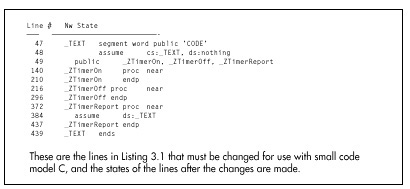
Altering the Zen timer for use in C’s large code model is a tad more complex, because in addition to the above changes, all functions, including the internal reference timing routines that are used to calculate overhead so it can be subtracted out, must be converted to far. Figure 3.3 shows the line numbers and new states of all lines from Listing 3.1 that must be changed in order to call the Zen timer from large code model C. Again, the line numbers are specific to the precision timer, but the long-period timer is very similar.
The full listings for the C-callable Zen timers are presented in Chapter K on the companion CD-ROM.
Watch Out for Optimizing Assemblers!
One important safety tip when modifying the Zen timer for use with large code model C code: Watch out for optimizing assemblers! TASM actually replaces
call far ptr ReferenceZTimerOnwith
push cs
call near ptr ReferenceZTimerOn(and likewise for ReferenceZTimerOff), which works
because ReferenceZTimerOn is in the same segment as the
calling code. This is normally a great optimization, being both smaller
and faster than a far call.
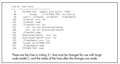
However, it’s not so great for the Zen timer, because our purpose in
calling the reference timing code is to determine exactly how much time
is taken by overhead code—including the far calls to
ZTimerOn and ZTimerOf! By converting the far
calls to push/near call pairs within the Zen timer module, TASM makes it
impossible to emulate exactly the overhead of the Zen timer, and makes
timings slightly (about 16 cycles on a 386) less accurate.
What’s the solution? Put the NOSMART directive at the
start of the Zen timer code. This directive instructs TASM to turn off
all optimizations, including converting far calls to push/near call
pairs. By the way, there is, to the best of my knowledge, no such
problem with MASM up through version 5.10A.
In my mind, the whole business of optimizing assemblers is a mixed blessing. In general, it’s nice to have the assembler shortening jumps and selecting sign-extended forms of instructions for you. On the other hand, the benefits of tricks like substituting push/near call pairs for far calls are relatively small, and those tricks can get in the way when complete control is needed. Sure, complete control is needed very rarely, but when it is, optimizing assemblers can cause subtle problems; I discovered TASM’s alteration of far calls only because I happened to view the code in the debugger, and you might want to do the same if you’re using a recent version of MASM.
I’ve tested the changes shown in Figures 3.2 and 3.3 with TASM and Borland C++ 4.0, and also with the latest MASM and Microsoft C/C++ compiler.
Further Reading
For those of you who wish to pursue the mechanics of code measurement further, one good article about measuring code performance with the 8253 timer is “Programming Insight: High-Performance Software Analysis on the IBM PC,” by Byron Sheppard, which appeared in the January, 1987 issue of Byte. For complete if somewhat cryptic information on the 8253 timer itself, I refer you to Intel’s Microsystem Components Handbook, which is also a useful reference for a number of other PC components, including the 8259 Programmable Interrupt Controller and the 8237 DMA Controller. For details about the way the 8253 is used in the PC, as well as a great deal of additional information about the PC’s hardware and BIOS resources, I suggest you consult IBM’s series of technical reference manuals for the PC, XT, AT, Model 30, and microchannel computers, such as the Models 50, 60, and 80.
For our purposes, however, it’s not critical that you understand exactly how the Zen timer works. All you really need to know is what the Zen timer can do and how to use it, and we’ve accomplished that in this chapter.
Armed with the Zen Timer, Onward and Upward
The Zen timer is not perfect. For one thing, the finest resolution to which it can measure an interval is at best about 1µs, a period of time in which a 66 MHz Pentium computer can execute as many as 132 instructions (although an 8088-based PC would be hard-pressed to manage two instructions in a microsecond). Another problem is that the timing code itself interferes with the state of the prefetch queue and processor cache at the start of the code being timed, because the timing code is not necessarily fetched and does not necessarily access memory in exactly the same time sequence as the code immediately preceding the code under measurement normally does. This prefetch effect can introduce as much as 3 to 4 µs of inaccuracy. Similarly, the state of the prefetch queue at the end of the code being timed affects how long the code that stops the timer takes to execute. Consequently, the Zen timer tends to be more accurate for longer code sequences, since the relative magnitude of the inaccuracy introduced by the Zen timer becomes less over longer periods.
Imperfections notwithstanding, the Zen timer is a good tool for exploring C code and x86 family assembly language, and it’s a tool we’ll use frequently for the remainder of this book.
Chapter 4 – In the Lair of the Cycle-Eaters
How the PC Hardware Devours Code Performance
This chapter, adapted from my earlier book, Zen of Assembly Language located on the companion CD-ROM, goes right to the heart of my philosophy of optimization: Understand where the time really goes when your code runs. That may sound ridiculously simple, but, as this chapter makes clear, it turns out to be a challenging task indeed, one that at times verges on black magic. This chapter is a long-time favorite of mine because it was the first—and to a large extent only—work that I know of that discussed this material, thereby introducing a generation of PC programmers to pedal-to-the-metal optimization.
This chapter focuses almost entirely on the first popular x86-family processor, the 8088. Some of the specific features and results that I cite in this chapter are no longer applicable to modern x86-family processors such as the 486 and Pentium, as I’ll point out later on when we discuss those processors. Nonetheless, the overall theme of this chapter—that understanding dimly-seen and poorly-documented code gremlins called cycle-eaters that lurk in your system is essential to performance programming—is every bit as valid today. Also, later chapters often refer back to the basic cycle-eaters described in this chapter, so this chapter is the foundation for the discussions of x86-family optimization to come. What’s more, the Zen timer remains an excellent tool with which to flush out and examine cycle-eaters, as we’ll see in later chapters, and this chapter is as good an illustration of how to use the Zen timer as you’re likely to find.
So, don’t take either the absolute or the relative execution times presented in this chapter as gospel for newer processors, and read on to later chapters to see how the cycle-eaters and optimization rules have changed over time, but do take the time to at least skim through this chapter to give yourself a good start on the material in the rest of this book.
Cycle-Eaters
Programming has many levels, ranging from the familiar (high-level languages, DOS calls, and the like) down to the esoteric things that lie on the shadowy edge of hardware-land. I call these cycle-eaters because, like the monsters in a bad 50s horror movie, they lurk in those shadows, taking their share of your program’s performance without regard to the forces of goodness or the U.S. Army. In this chapter, we’re going to jump right in at the lowest level by examining the cycle-eaters that live beneath the programming interface; that is, beneath your application, DOS, and BIOS—in fact, beneath the instruction set itself.
Why start at the lowest level? Simply because cycle-eaters affect the performance of all assembler code, and yet are almost unknown to most programmers. A full understanding of code optimization requires an understanding of cycle-eaters and their implications. That’s no simple task, and in fact it is in precisely that area that most books and articles about assembly programming fall short.
Nearly all literature on assembly programming discusses only the programming interface: the instruction set, the registers, the flags, and the BIOS and DOS calls. Those topics cover the functionality of assembly programs most thoroughly—but it’s performance above all else that we’re after. No one ever tells you about the raw stuff of performance, which lies beneath the programming interface, in the dimly-seen realm—populated by instruction prefetching, dynamic RAM refresh, and wait states—where software meets hardware. This area is the domain of hardware engineers, and is almost never discussed as it relates to code performance. And yet it is only by understanding the mechanisms operating at this level that we can fully understand and properly improve the performance of our code.
Which brings us to cycle-eaters.
The Nature of Cycle-Eaters
Cycle-eaters are gremlins that live on the bus or in peripherals (and sometimes within the CPU itself), slowing the performance of PC code so that it doesn’t execute at full speed. Most cycle-eaters (and all of those haunting the older Intel processors) live outside the CPU’s Execution Unit, where they can only affect the CPU when the CPU performs a bus access (a memory or I/O read or write). Once your code and data are already inside the CPU, those cycle-eaters can no longer be a problem. Only on the 486 and Pentium CPUs will you find cycle-eaters inside the chip, as we’ll see in later chapters.
The nature and severity of the cycle-eaters vary enormously from processor to processor, and (especially) from memory architecture to memory architecture. In order to understand them all, we need first to understand the simplest among them, those that haunted the original 8088-based IBM PC. Later on in this book, I’ll be better able to explain the newer generation of cycle-eaters in terms of those ancestral cycle-eaters—but we have to get the groundwork down first.
The 8088’s Ancestral Cycle-Eaters
Internally, the 8088 is a 16-bit processor, capable of running at full speed at all times—unless external data is required. External data must traverse the 8088’s external data bus and the PC’s data bus one byte at a time to and from peripherals, with cycle-eaters lurking along every step of the way. What’s more, external data includes not only memory operands but also instruction bytes, so even instructions with no memory operands can suffer from cycle-eaters. Since some of the 8088’s fastest instructions are register-only instructions, that’s important indeed.
The major cycle-eaters are:
- The 8088’s 8-bit external data bus.
- The prefetch queue.
- Dynamic RAM refresh.
- Wait states, notably display memory wait states and, in the AT and 80386 computers, system memory wait states.
The locations of these cycle-eaters in the primordial 8088-based PC are shown in Figure 4.1. We’ll cover each of the cycle-eaters in turn in this chapter. The material won’t be easy since cycle-eaters are among the most subtle aspects of assembly programming. By the same token, however, this will be one of the most important and rewarding chapters in this book. Don’t worry if you don’t catch everything in this chapter, but do read it all even if the going gets a bit tough. Cycle-eaters play a key role in later chapters, so some familiarity with them is highly desirable.
The 8-Bit Bus Cycle-Eater
Look! Down on the motherboard! It’s a 16-bit processor! It’s an 8-bit processor! It’s…
…an 8088!
Fans of the 8088 call it a 16-bit processor. Fans of other 16-bit processors call the 8088 an 8-bit processor. The truth of the matter is that the 8088 is a 16-bit processor that often performs like an 8-bit processor.
The 8088 is internally a full 16-bit processor, equivalent to an 8086. (In fact, the 8086 is identical to the 8088, except that it has a full 16-bit bus. The 8088 is basically the poor man’s 8086, because it allows a cheaper—albeit slower—system to be built, thanks to the half-sized bus.) In terms of the instruction set, the 8088 is clearly a 16-bit processor, capable of performing any given 16-bit operation—addition, subtraction, even multiplication or division—with a single instruction. Externally, however, the 8088 is unequivocally an 8-bit processor, since the external data bus is only 8 bits wide. In other words, the programming interface is 16 bits wide, but the hardware interface is only 8 bits wide, as shown in Figure 4.2. The result of this mismatch is simple: Word-sized data can be transferred between the 8088 and memory or peripherals at only one-half the maximum rate of the 8086, which is to say one-half the maximum rate for which the Execution Unit of the 8088 was designed.
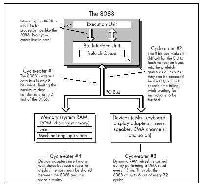
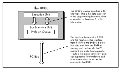
As shown in Figure 4.1, the 8-bit bus cycle-eater lies squarely on the 8088’s external data bus. Technically, it might be more accurate to place this cycle-eater in the Bus Interface Unit, which breaks 16-bit memory accesses into paired 8-bit accesses, but it is really the limited width of the external data bus that constricts data flow into and out of the 8088. True, the original PC’s bus is also only 8 bits wide, but that’s just to match the 8088’s 8-bit bus; even if the PC’s bus were 16 bits wide, data could still pass into and out of the 8088 chip itself only 1 byte at a time.
Each bus access by the 8088 takes 4 clock cycles, or 0.838 µs in the 4.77 MHz PC, and transfers 1 byte. That means that the maximum rate at which data can be transferred into and out of the 8088 is 1 byte every 0.838 µs. While 8086 bus accesses also take 4 clock cycles, each 8086 bus access can transfer either 1 byte or 1 word, for a maximum transfer rate of 1 word every 0.838 µs. Consequently, for word-sized memory accesses, the 8086 has an effective transfer rate of 1 byte every 0.419 µs. By contrast, every word-sized access on the 8088 requires two 4-cycle-long bus accesses, one for the high byte of the word and one for the low byte of the word. As a result, the 8088 has an effective transfer rate for word-sized memory accesses of just 1 word every 1.676 µs—and that, in a nutshell, is the 8-bit bus cycle-eater.
A related cycle-eater lurks beneath the 386SX chip, which is a 32-bit processor internally with only a 16-bit path to system memory. The numbers are different, but the way the cycle-eater operates is exactly the same. AT-compatible systems have 16-bit data buses, which can access a full 16-bit word at a time. The 386SX can process 32 bits (a doubleword) at a time, however, and loses a lot of time fetching that doubleword from memory in two halves.
The Impact of the 8-Bit Bus Cycle-Eater
One obvious effect of the 8-bit bus cycle-eater is that word-sized accesses to memory operands on the 8088 take 4 cycles longer than byte-sized accesses. That’s why the official instruction timings indicate that for code running on an 8088 an additional 4 cycles are required for every word-sized access to a memory operand. For instance,
mov ax,word ptr [MemVar]takes 4 cycles longer to read the word at address MemVar
than
mov al,byte ptr [MemVar]takes to read the byte at address MemVar. (Actually, the
difference between the two isn’t very likely to be exactly 4 cycles, for
reasons that will become clear once we discuss the prefetch queue and
dynamic RAM refresh cycle-eaters later in this chapter.)
What’s more, in some cases one instruction can perform multiple word-sized accesses, incurring that 4-cycle penalty on each access. For example, adding a value to a word-sized memory variable requires two word-sized accesses—one to read the destination operand from memory prior to adding to it, and one to write the result of the addition back to the destination operand—and thus incurs not one but two 4-cycle penalties. As a result
add word ptr [MemVar],axtakes about 8 cycles longer to execute than:
add byte ptr [MemVar],alString instructions can suffer from the 8-bit bus cycle-eater to a
greater extent than other instructions. Believe it or not, a single
REP MOVSW instruction can lose as much as 131,070
word-sized memory accesses x 4 cycles, or 524,280 cycles to the
8-bit bus cycle-eater! In other words, one 8088 instruction (admittedly,
an instruction that does a great deal) can take over one-tenth of a
second longer on an 8088 than on an 8086, simply because of the 8-bit
bus. One-tenth of a second! That’s a phenomenally long time in
computer terms; in one-tenth of a second, the 8088 can perform more than
50,000 additions and subtractions.
The upshot of all this is simply that the 8088 can transfer word-sized data to and from memory at only half the speed of the 8086, which inevitably causes performance problems when coupled with an Execution Unit that can process word-sized data every bit as quickly as an 8086. These problems show up with any code that uses word-sized memory operands. More ominously, as we will see shortly, the 8-bit bus cycle-eater can cause performance problems with other sorts of code as well.
What to Do about the 8-Bit Bus Cycle-Eater?
The obvious implication of the 8-bit bus cycle-eater is that
byte-sized memory variables should be used whenever possible. After all,
the 8088 performs byte-sized memory accesses just as quickly as
the 8086. For instance, Listing 4.1, which uses a byte-sized memory
variable as a loop counter, runs in 10.03 s per loop. That’s 20 percent
faster than the 12.05 µs per loop execution time of Listing 4.2, which
uses a word-sized counter. Why the difference in execution times? Simply
because each word-sized DEC performs 4 byte-sized memory
accesses (two to read the word-sized operand and two to write the result
back to memory), while each byte-sized DEC performs only 2
byte-sized memory accesses in all.
LISTING 4.1 LST4-1.ASM
; Measures the performance of a loop which uses a
; byte-sized memory variable as the loop counter.
;
jmp Skip
;
Counter db 100
;
Skip:
call ZTimerOn
LoopTop:
dec [Counter]
jnz LoopTop
call ZTimerOffLISTING 4.2 LST4-2.ASM
; Measures the performance of a loop which uses a
; word-sized memory variable as the loop counter.
;
jmp Skip
;
Counter dw 100
;
Skip:
call ZTimerOn
LoopTop:
dec [Counter]
jnz LoopTop
call ZTimerOffI’d like to make a brief aside concerning code optimization in the
listings in this book. Throughout this book I’ve modeled the sample code
after working code so that the timing results are applicable to
real-world programming. In Listings 4.1 and 4.2, for example, I could
have shown a still greater advantage for byte-sized operands simply by
performing 1,000 DEC instructions in a row, with no
branching at all. However, DEC instructions don’t exist in
a vacuum, so in the listings I used code that both decremented the
counter and tested the result. The difference is that between
decrementing a memory location (simply an instruction) and using a loop
counter (a functional instruction sequence). If you come across code in
this book that seems less than optimal, it’s simply due to my desire to
provide code that’s relevant to real programming problems. On the other
hand, optimal code is an elusive thing indeed; by no means should you
assume that the code in this book is ideal! Examine it, question it, and
improve upon it, for an inquisitive, skeptical mind is an important part
of the Zen of assembly optimization.
Back to the 8-bit bus cycle-eater. As I’ve said, in 8088 work you should strive to use byte-sized memory variables whenever possible. That does not mean that you should use 2 byte-sized memory accesses to manipulate a word-sized memory variable in preference to 1 word-sized memory access, as, for instance,
mov dl,byte ptr [MemVar]
mov dh,byte ptr [MemVar+1]versus:
mov dx,word ptr [MemVar]Recall that every access to a memory byte takes at least 4 cycles; that limitation is built right into the 8088. The 8088 is also built so that the second byte-sized memory access to a 16-bit memory variable takes just those 4 cycles and no more. There’s no way you can manipulate the second byte of a word-sized memory variable faster with a second separate byte-sized instruction in less than 4 cycles. As a matter of fact, you’re bound to access that second byte much more slowly with a separate instruction, thanks to the overhead of instruction fetching and execution, address calculation, and the like.
For example, consider Listing 4.3, which performs 1,000 word-sized
reads from memory. This code runs in 3.77 µs per word read on a 4.77 MHz
8088. That’s 45 percent faster than the 5.49 µs per word read of Listing
4.4, which reads the same 1,000 words as Listing 4.3 but does so with
2,000 byte-sized reads. Both listings perform exactly the same number of
memory accesses—2,000 accesses, each byte-sized, as all 8088 memory
accesses must be. (Remember that the Bus Interface Unit must perform two
byte-sized memory accesses in order to handle a word-sized memory
operand.) However, Listing 4.3 is considerably faster because it expends
only 4 additional cycles to read the second byte of each word, while
Listing 4.4 performs a second LODSB, requiring 13 cycles,
to read the second byte of each word.
LISTING 4.3 LST4-3.ASM
; Measures the performance of reading 1,000 words
; from memory with 1,000 word-sized accesses.
;
sub si,si
mov cx,1000
call ZTimerOn
rep lodsw
call ZTimerOffLISTING 4.4 LST4-4.ASM
; Measures the performance of reading 1000 words
; from memory with 2,000 byte-sized accesses.
;
sub si,si
mov cx,2000
call ZTimerOn
rep lodsb
call ZTimerOffIn short, if you must perform a 16-bit memory access, let the 8088 break the access into two byte-sized accesses for you. The 8088 is more efficient at that task than your code can possibly be.
Word-sized variables should be stored in registers to the greatest feasible extent, since registers are inside the 8088, where 16-bit operations are just as fast as 8-bit operations because the 8-bit cycle-eater can’t get at them. In fact, it’s a good idea to keep as many variables of all sorts in registers as you can. Instructions with register-only operands execute very rapidly, partially because they avoid both the time-consuming memory accesses and the lengthy address calculations associated with memory operands.
There is yet another reason why register operands are preferable to memory operands, and it’s an unexpected effect of the 8-bit bus cycle-eater. Instructions with only register operands tend to be shorter (in terms of bytes) than instructions with memory operands, and when it comes to performance, shorter is usually better. In order to explain why that is true and how it relates to the 8-bit bus cycle-eater, I must diverge for a moment.
For the last few pages, you may well have been thinking that the 8-bit bus cycle-eater, while a nuisance, doesn’t seem particularly subtle or difficult to quantify. After all, any instruction reference tells us exactly how many cycles each instruction loses to the 8-bit bus cycle-eater, doesn’t it?
Yes and no. It’s true that in general we know approximately how much longer a given instruction will take to execute with a word-sized memory operand than with a byte-sized operand, although the dynamic RAM refresh and wait state cycle-eaters (which I’ll cover a little later) can raise the cost of the 8-bit bus cycle-eater considerably. However, all word-sized memory accesses lose 4 cycles to the 8-bit bus cycle-eater, and there’s one sort of word-sized memory access we haven’t discussed yet: instruction fetching. The ugliest manifestation of the 8-bit bus cycle-eater is in fact the prefetch queue cycle-eater.
The Prefetch Queue Cycle-Eater
In an 8088 context, here’s the prefetch queue cycle-eater in a nutshell: The 8088’s 8-bit external data bus keeps the Bus Interface Unit from fetching instruction bytes as fast as the 16-bit Execution Unit can execute them, so the Execution Unit often lies idle while waiting for the next instruction byte to be fetched.
Exactly why does this happen? Recall that the 8088 is an 8086 internally, but accesses word-sized memory data at only one-half the maximum rate of the 8086 due to the 8088’s 8-bit external data bus. Unfortunately, instructions are among the word-sized data the 8086 fetches, meaning that the 8088 can fetch instructions at only one-half the speed of the 8086. On the other hand, the 8086-equivalent Execution Unit of the 8088 can execute instructions every bit as fast as the 8086. The net result is that the Execution Unit burns up instruction bytes much faster than the Bus Interface Unit can fetch them, and ends up idling while waiting for instructions bytes to arrive.
The BIU can fetch instruction bytes at a maximum rate of one byte every 4 cycles—and that 4-cycle per instruction byte rate is the ultimate limit on overall instruction execution time, regardless of EU speed. While the EU may execute a given instruction that’s already in the prefetch queue in less than 4 cycles per byte, over time the EU can’t execute instructions any faster than they can arrive—and they can’t arrive faster than 1 byte every 4 cycles.
Clearly, then, the prefetch queue cycle-eater is nothing more than one aspect of the 8-bit bus cycle-eater. 8088 code often runs at less than the Execution Unit’s maximum speed because the 8-bit data bus can’t keep up with the demand for instruction bytes. That’s straightforward enough—so why all the fuss about the prefetch queue cycle-eater?
What makes the prefetch queue cycle-eater tricky is that it’s undocumented and unpredictable. That is, with a word-sized memory access, such as
mov [bx],axit’s well-documented that an extra 4 cycles will always be required to write the upper byte of AX to memory. Not so with the prefetch queue cycle-eater lurking nearby. For instance, the instructions
shr ax,1
shr ax,1
shr ax,1
shr ax,1
shr ax,1should execute in 10 cycles, since each SHR takes 2
cycles to execute, according to Intel’s specifications. Those
specifications contain Intel’s official instruction execution times, but
in this case—and in many others—the specifications are drastically
wrong. Why? Because they describe execution time once an instruction
reaches the prefetch queue. They say nothing about whether a given
instruction will be in the prefetch queue when it’s time for that
instruction to run, or how long it will take that instruction to reach
the prefetch queue if it’s not there already. Thanks to the low
performance of the 8088’s external data bus, that’s a glaring
omission—but, alas, an unavoidable one. Let’s look at why the official
execution times are wrong, and why that can’t be helped.
Official Execution Times Are Only Part of the Story
The sequence of 5 SHR instructions in the last example
is 10 bytes long. That means that it can never execute in less than 24
cycles even if the 4-byte prefetch queue is full when it starts, since 6
instruction bytes would still remain to be fetched, at 4 cycles per
fetch. If the prefetch queue is empty at the start, the sequence
could take 40 cycles. In short, thanks to instruction fetching,
the code won’t run at its documented speed, and could take up to four
times longer than it is supposed to.
Why does Intel document Execution Unit execution time rather than overall instruction execution time, which includes both instruction fetch time and Execution Unit (EU) execution time? Well, instruction fetching isn’t performed as part of instruction execution by the Execution Unit, but instead is carried on in parallel by the Bus Interface Unit (BIU) whenever the external data bus isn’t in use or whenever the EU runs out of instruction bytes to execute. Sometimes the BIU is able to use spare bus cycles to prefetch instruction bytes before the EU needs them, so in those cases instruction fetching takes no time at all, practically speaking. At other times the EU executes instructions faster than the BIU can fetch them, and instruction fetching then becomes a significant part of overall execution time. As a result, the effective fetch time for a given instruction varies greatly depending on the code mix preceding that instruction. Similarly, the state in which a given instruction leaves the prefetch queue affects the overall execution time of the following instructions.
As we’ll see later, other cycle-eaters, such as DRAM refresh and display memory wait states, can cause prefetching variations even during different executions of the same code sequence. Given that, it’s meaningless to talk about the prefetch time of a given instruction except in the context of a specific code sequence.
So now you know why the official instruction execution times are often wrong, and why Intel can’t provide better specifications. You also know now why it is that you must time your code if you want to know how fast it really is.
There Is No Such Beast as a True Instruction Execution Time
The effect of the code preceding an instruction on the execution time of that instruction makes the Zen timer trickier to use than you might expect, and complicates the interpretation of the results reported by the Zen timer. For one thing, the Zen timer is best used to time code sequences that are more than a few instructions long; below 10µs or so, prefetch queue effects and the limited resolution of the clock driving the timer can cause problems.
Some slight prefetch queue-induced inaccuracy usually exists even when the Zen timer is used to time longer code sequences, since the calls to the Zen timer usually alter the code’s prefetch queue from its normal state. (Branches—jumps, calls, returns and the like—empty the prefetch queue.) Ideally, the Zen timer is used to measure the performance of an entire subroutine, so the prefetch queue effects of the branches at the start and end of the subroutine are similar to the effects of the calls to the Zen timer when you’re measuring the subroutine’s performance.
Another way in which the prefetch queue cycle-eater complicates the use of the Zen timer involves the practice of timing the performance of a few instructions over and over. I’ll often repeat one or two instructions 100 or 1,000 times in a row in listings in this book in order to get timing intervals that are long enough to provide reliable measurements. However, as we just learned, the actual performance of any 8088 instruction depends on the code mix preceding any given use of that instruction, which in turn affects the state of the prefetch queue when the instruction starts executing. Alas, the execution time of an instruction preceded by dozens of identical instructions reflects just one of many possible prefetch states (and not a very likely state at that), and some of the other prefetch states may well produce distinctly different results.
For example, consider the code in Listings 4.5 and 4.6. Listing 4.5
shows our familiar SHR case. Here, because the prefetch
queue is always empty, execution time should work out to about 4 cycles
per byte, or 8 cycles per SHR, as shown in Figure 4.3.
(Figure 4.3 illustrates the relationship between instruction fetching
and execution in a simplified way, and is not intended to show the exact
timings of 8088 operations.) That’s quite a contrast to the official
2-cycle execution time of SHR. In fact, the Zen timer
reports that Listing 4.5 executes in 1.81µs per byte, or slightly
more than 4 cycles per byte. (The extra time is the result of
the dynamic RAM refresh cycle-eater, which we’ll discuss shortly.) Going
by Listing 4.5, we would conclude that the “true” execution time of
SHR is 8.64 cycles.
LISTING 4.5 LST4-5.ASM
; Measures the performance of 1,000 SHR instructions
; in a row. Since SHR executes in 2 cycles but is
; 2 bytes long, the prefetch queue is always empty,
; and prefetching time determines the overall
; performance of the code.
;
call ZTimerOn
rept 1000
shr ax,1
endm
call ZTimerOffLISTING 4.6 LST4-6.ASM
; Measures the performance of 1,000 MUL/SHR instruction
; pairs in a row. The lengthy execution time of MUL
; should keep the prefetch queue from ever emptying.
;
mov cx,1000
sub ax,ax
call ZTimerOn
rept 1000
mul ax
shr ax,1
endm
call ZTimerOff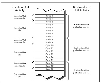
Now let’s examine Listing 4.6. Here each SHR follows a
MUL instruction. Since MUL instructions take
so long to execute that the prefetch queue is always full when they
finish, each SHR should be ready and waiting in the
prefetch queue when the preceding MUL ends. As a result,
we’d expect that each SHR would execute in 2 cycles;
together with the 118-cycle execution time of multiplying 0 times 0, the
total execution time should come to 120 cycles per SHR/MUL
pair, as shown in Figure 4.4. And, by God, when we run Listing 4.6 we
get an execution time of 25.14 µs per SHR/MUL pair, or
exactly 120 cycles! According to these results, the “true”
execution time of SHR would seem to be 2 cycles, quite a
change from the conclusion we drew from Listing 4.5.
The key point is this: We’ve seen one code sequence in which
SHR took 8-plus cycles to execute, and another in which it
took only 2 cycles. Are we talking about two different forms of
SHR here? Of course not—the difference is purely a
reflection of the differing states in which the preceding code left the
prefetch queue. In Listing 4.5, each SHR after the first
few follows a slew of other SHR instructions which have
sucked the prefetch queue dry, so overall performance reflects
instruction fetch time. By contrast, each SHR in Listing
4.6 follows a MUL instruction which leaves the prefetch
queue full, so overall performance reflects Execution Unit execution
time.
Clearly, either instruction fetch time or Execution Unit execution time—or even a mix of the two, if an instruction is partially prefetched—can determine code performance. Some people operate under a rule of thumb by which they assume that the execution time of each instruction is 4 cycles times the number of bytes in the instruction. While that’s often true for register-only code, it frequently doesn’t hold for code that accesses memory. For one thing, the rule should be 4 cycles times the number of memory accesses, not instruction bytes, since all accesses take 4 cycles on the 8088-based PC. For another, memory-accessing instructions often have slower Execution Unit execution times than the 4 cycles per memory access rule would dictate, because the 8088 isn’t very fast at calculating memory addresses. Also, the 4 cycles per instruction byte rule isn’t true for register-only instructions that are already in the prefetch queue when the preceding instruction ends.
The truth is that it never hurts performance to reduce either the
cycle count or the byte count of a given bit of code, but there’s no
guarantee that one or the other will improve performance either. For
example, consider Listing 4.7, which consists of a series of 4-cycle,
2-byte MOV AL,0 instructions, and which executes at the
rate of 1.81 µs per instruction. Now consider Listing 4.8, which
replaces the 4-cycle MOV AL,0 with the 3-cycle (but still
2-byte) SUB AL,AL, Despite its 1-cycle-per-instruction
advantage, Listing 4.8 runs at exactly the same speed as Listing 4.7.
The reason: Both instructions are 2 bytes long, and in both cases it is
the 8-cycle instruction fetch time, not the 3 or 4-cycle Execution Unit
execution time, that limits performance.
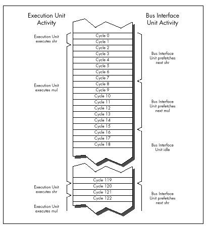
LISTING 4.7 LST4-7.ASM
; Measures the performance of repeated MOV AL,0 instructions,
; which take 4 cycles each according to Intel's official
; specifications.
;
sub ax,ax
call ZTimerOn
rept 1000
mov al,0
endm
call ZTimerOffLISTING 4.8 LST4-8.ASM
; Measures the performance of repeated SUB AL,AL instructions,
; which take 3 cycles each according to Intel's official
; specifications.
;
sub ax,ax
call ZTimerOn
rept 1000
sub al,al
endm
call ZTimerOffAs you can see, it’s easy to be drawn into thinking you’re saving cycles when you’re not. You can only improve the performance of a specific bit of code by reducing the factor—either instruction fetch time or execution time, or sometimes a mix of the two—that’s limiting the performance of that code.
In case you missed it in all the excitement, the variability of prefetching means that our method of testing performance by executing 1,000 instructions in a row by no means produces “true” instruction execution times, any more than the official execution times in the Intel manuals are “true” times. The fact of the matter is that a given instruction takes at least as long to execute as the time given for it in the Intel manuals, but may take as much as 4 cycles per byte longer, depending on the state of the prefetch queue when the preceding instruction ends.
What we really want is to know how long useful working code takes to run, not how long a single instruction takes, and the Zen timer gives us the tool we need to gather that information. Granted, it would be easier if we could just add up neatly documented instruction execution times—but that’s not going to happen. Without actually measuring the performance of a given code sequence, you simply don’t know how fast it is. For crying out loud, even the people who designed the 8088 at Intel couldn’t tell you exactly how quickly a given 8088 code sequence executes on the PC just by looking at it! Get used to the idea that execution times are only meaningful in context, learn the rules of thumb in this book, and use the Zen timer to measure your code.
Approximating Overall Execution Times
Don’t think that because overall instruction execution time is
determined by both instruction fetch time and Execution Unit execution
time, the two times should be added together when estimating
performance. For example, practically speaking, each SHR in
Listing 4.5 does not take 8 cycles of instruction fetch time plus 2
cycles of Execution Unit execution time to execute. Figure 4.3 shows
that while a given SHR is executing, the fetch of the next
SHR is starting, and since the two operations are
overlapped for 2 cycles, there’s no sense in charging the time to both
instructions. You could think of the extra instruction fetch time for
SHR in Listing 4.5 as being 6 cycles, which yields an
overall execution time of 8 cycles when added to the 2 cycles of
Execution Unit execution time.
Alternatively, you could think of each SHR in Listing
4.5 as taking 8 cycles to fetch, and then executing in effectively 0
cycles while the next SHR is being fetched. Whichever
perspective you prefer is fine. The important point is that the time
during which the execution of one instruction and the fetching of the
next instruction overlap should only be counted toward the overall
execution time of one of the instructions. For all intents and purposes,
one of the two instructions runs at no performance cost whatsoever while
the overlap exists.
As a working definition, we’ll consider the execution time of a given instruction in a particular context to start when the first byte of the instruction is sent to the Execution Unit and end when the first byte of the next instruction is sent to the EU.
What to Do about the Prefetch Queue Cycle-Eater?
Reducing the impact of the prefetch queue cycle-eater is one of the overriding principles of high-performance assembly code. How can you do this? One effective technique is to minimize access to memory operands, since such accesses compete with instruction fetching for precious memory accesses. You can also greatly reduce instruction fetch time simply by your choice of instructions: Keep your instructions short. Less time is required to fetch instructions that are 1 or 2 bytes long than instructions that are 5 or 6 bytes long. Reduced instruction fetching lowers minimum execution time (minimum execution time is 4 cycles times the number of instruction bytes) and often leads to faster overall execution.
While short instructions minimize overall prefetch time, ironically
they actually often suffer more from the prefetch queue bottleneck than
do long instructions. Short instructions generally have such fast
execution times that they drain the prefetch queue despite their small
size. For example, consider the SHR of Listing 4.5, which
runs at only 25 percent of its Execution Unit execution time even though
it’s only 2 bytes long, thanks to the prefetch queue bottleneck. Short
instructions are nonetheless generally faster than long instructions,
thanks to the combination of fewer instruction bytes and faster
Execution Unit execution times, and should be used as much as
possible—just don’t expect them to run at their “official” documented
speeds.
More than anything, the above rules mean using the registers as heavily as possible, both because register-only instructions are short and because they don’t perform memory accesses to read or write operands. However, using the registers is a rule of thumb, not a commandment. In some circumstances, it may actually be faster to access memory. (The look-up table technique is one such case.) What’s more, the performance of the prefetch queue (and hence the performance of each instruction) differs from one code sequence to the next, and can even differ during different executions of the same code sequence.
All in all, writing good assembler code is as much an art as a science. As a result, you should follow the rules of thumb described here—and then time your code to see how fast it really is. You should experiment freely, but always remember that actual, measured performance is the bottom line.
Holding Up the 8088
In this chapter I’ve taken you further and further into the depths of the PC, telling you again and again that you must understand the computer at the lowest possible level in order to write good code. At this point, you may well wonder, “Have we gotten low enough?”
Not quite yet. The 8-bit bus and prefetch queue cycle-eaters are low-level indeed, but we’ve one level yet to go. Dynamic RAM refresh and wait states—our next topics—together form the lowest level at which the hardware of the PC affects code performance. Below this level, the PC is of interest only to hardware engineers.
Before we begin our discussion of dynamic RAM refresh, let’s step back for a moment to take an overall look at this lowest level of cycle-eaters. In truth, the distinctions between wait states and dynamic RAM refresh don’t much matter to a programmer. What is important is that you understand this: Under certain circumstances, devices on the PC bus can stop the CPU for 1 or more cycles, making your code run more slowly than it seemingly should.
Unlike all the cycle-eaters we’ve encountered so far, wait states and dynamic RAM refresh are strictly external to the CPU, as was shown in Figure 4.1. Adapters on the PC’s bus, such as video and memory cards, can insert wait states on any bus access, the idea being that they won’t be able to complete the access properly unless the access is stretched out. Likewise, the channel of the DMA controller dedicated to dynamic RAM refresh can request control of the bus at any time, although the CPU must relinquish the bus before the DMA controller can take over. This means that your code can’t directly control wait states or dynamic RAM refresh. However, code can sometimes be designed to minimize the effects of these cycle-eaters, and even when the cycle-eaters slow your code without there being a thing in the world you can do about it, you’re still better off understanding that you’re losing performance and knowing why your code doesn’t run as fast as it’s supposed to than you were programming in ignorance.
Let’s start with DRAM refresh, which affects the performance of every program that runs on the PC.
Dynamic RAM Refresh: The Invisible Hand
Dynamic RAM (DRAM) refresh is sort of an act of God. By that I mean that DRAM refresh invisibly and inexorably steals a certain fraction of all available memory access time from your programs, when they are accessing memory for code and data. (When they are accessing cache on more recent processors, theoretically the DRAM refresh cycle-eater doesn’t come into play, but there are other cycle-eaters waiting to prey on cache-bound programs.) While you could stop DRAM refresh, you wouldn’t want to since that would be a sure prescription for crashing your computer. In the end, thanks to DRAM refresh, almost all code runs a bit slower on the PC than it otherwise would, and that’s that.
A bit of background: A static RAM (SRAM) chip is a memory chip that retains its contents indefinitely so long as power is maintained. By contrast, each of several blocks of bits in a dynamic RAM (DRAM) chip retains its contents for only a short time after it’s accessed for a read or write. In order to get a DRAM chip to store data for an extended period, each of the blocks of bits in that chip must be accessed regularly, so that the chip’s stored data is kept refreshed and valid. So long as this is done often enough, a DRAM chip will retain its contents indefinitely.
All of the PC’s system memory consists of DRAM chips. Each DRAM chip in the PC must be completely refreshed about once every four milliseconds in order to ensure the integrity of the data it stores. Obviously, it’s highly desirable that the memory in the PC retain the correct data indefinitely, so each DRAM chip in the PC must always be refreshed within 4 ms of the last refresh. Since there’s no guarantee that a given program will access each and every DRAM block once every 4 ms, the PC contains special circuitry and programming for providing DRAM refresh.
How DRAM Refresh Works in the PC
On the original 8088-based IBM PC, timer 1 of the 8253 timer chip is programmed at power-up to generate a signal once every 72 cycles, or once every 15.08µs. That signal goes to channel 0 of the 8237 DMA controller, which requests the bus from the 8088 upon receiving the signal. (DMA stands for direct memory access, the ability of a device other than the 8088 to control the bus and access memory directly, without any help from the 8088.) As soon as the 8088 is between memory accesses, it gives control of the bus to the 8237, which in conjunction with special circuitry on the PC’s motherboard then performs a single 4-cycle read access to 1 of 256 possible addresses, advancing to the next address on each successive access. (The read access is only for the purpose of refreshing the DRAM; the data that is read isn’t used.)
The 256 addresses accessed by the refresh DMA accesses are arranged so that taken together they properly refresh all the memory in the PC. By accessing one of the 256 addresses every 15.08 µs, all of the PC’s DRAM is refreshed in 256 x 15.08 µs, or 3.86 ms, which is just about the desired 4 ms time I mentioned earlier. (Only the first 640K of memory is refreshed in the PC; video adapters and other adapters above 640K containing memory that requires refreshing must provide their own DRAM refresh in pre-AT systems.)
Don’t sweat the details here. The important point is this: For at least 4 out of every 72 cycles, the original PC’s bus is given over to DRAM refresh and is not available to the 8088, as shown in Figure 4.5. That means that as much as 5.56 percent of the PC’s already inadequate bus capacity is lost. However, DRAM refresh doesn’t necessarily stop the 8088 in its tracks for 4 cycles. The Execution Unit of the 8088 can keep processing while DRAM refresh is occurring, unless the EU needs to access memory. Consequently, DRAM refresh can slow code performance anywhere from 0 percent to 5.56 percent (and actually a bit more, as we’ll see shortly), depending on the extent to which DRAM refresh occupies cycles during which the 8088 would otherwise be accessing memory.
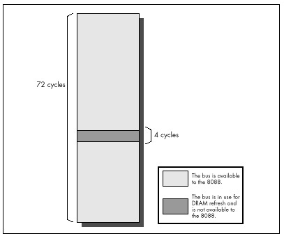
The Impact of DRAM Refresh
Let’s look at examples from opposite ends of the spectrum in terms of
the impact of DRAM refresh on code performance. First, consider the
series of MUL instructions in Listing 4.9. Since a 16-bit
MUL on the 8088 executes in between 118 and 133 cycles and
is only 2 bytes long, there should be plenty of time for the prefetch
queue to fill after each instruction, even after DRAM refresh has taken
its slice of memory access time. Consequently, the prefetch queue should
be able to keep the Execution Unit well-supplied with instruction bytes
at all times. Since Listing 4.9 uses no memory operands, the Execution
Unit should never have to wait for data from memory, and DRAM refresh
should have no impact on performance. (Remember that the Execution Unit
can operate normally during DRAM refreshes so long as it doesn’t need to
request a memory access from the Bus Interface Unit.)
LISTING 4.9 LST4-9.ASM
; Measures the performance of repeated MUL instructions,
; which allow the prefetch queue to be full at all times,
; to demonstrate a case in which DRAM refresh has no impact
; on code performance.
;
sub ax,ax
call ZTimerOn
rept 1000
mul ax
endm
call ZTimerOffRunning Listing 4.9, we find that each MUL executes in
24.72 µs, or exactly 118 cycles. Since that’s the shortest time in which
MUL can execute, we can see that no performance is lost to
DRAM refresh. Listing 4.9 clearly illustrates that DRAM refresh only
affects code performance when a DRAM refresh forces the Execution Unit
of the 8088 to wait for a memory access.
Now let’s look at the series of SHR instructions shown
in Listing 4.10. Since SHR executes in 2 cycles but is 2
bytes long, the prefetch queue should be empty while Listing 4.10
executes, with the 8088 prefetching instruction bytes non-stop. As a
result, the time per instruction of Listing 4.10 should precisely
reflect the time required to fetch the instruction bytes.
LISTING 4.10 LST4-10.ASM
; Measures the performance of repeated SHR instructions,
; which empty the prefetch queue, to demonstrate the
; worst-case impact of DRAM refresh on code performance.
;
call ZTimerOn
rept 1000
shr ax,1
endm
call ZTimerOffSince 4 cycles are required to read each instruction byte, we’d
expect each SHR to execute in 8 cycles, or 1.676 µs, if
there were no DRAM refresh. In fact, each SHR in Listing
4.10 executes in 1.81 µs, indicating that DRAM refresh is taking 7.4
percent of the program’s execution time. That’s nearly 2 percent more
than our worst-case estimate of the loss to DRAM refresh overhead! In
fact, the result indicates that DRAM refresh is stealing not 4, but 5.33
cycles out of every 72 cycles. How can this be?
The answer is that a given DRAM refresh can actually hold up CPU
memory accesses for as many as 6 cycles, depending on the timing of the
DRAM refresh’s DMA request relative to the 8088’s internal instruction
execution state. When the code in Listing 4.10 runs, each DRAM refresh
holds up the CPU for either 5 or 6 cycles, depending on where the 8088
is in executing the current SHR instruction when the
refresh request occurs. Now we see that things can get even worse than
we thought: DRAM refresh can steal as much as 8.33 percent of
available memory access time—6 out of every 72 cycles—from the
8088.
Which of the two cases we’ve examined reflects reality? While either case can happen, the latter case—significant performance reduction, ranging as high as 8.33 percent—is far more likely to occur. This is especially true for high-performance assembly code, which uses fast instructions that tend to cause non-stop instruction fetching.
What to Do About the DRAM Refresh Cycle-Eater?
Hmmm. When we discovered the prefetch queue cycle-eater, we learned to use short instructions. When we discovered the 8-bit bus cycle-eater, we learned to use byte-sized memory operands whenever possible, and to keep word-sized variables in registers. What can we do to work around the DRAM refresh cycle-eater?
Nothing.
As I’ve said before, DRAM refresh is an act of God. DRAM refresh is a fundamental, unchanging part of the PC’s operation, and there’s nothing you or I can do about it. If refresh were any less frequent, the reliability of the PC would be compromised, so tinkering with either timer 1 or DMA channel 0 to reduce DRAM refresh overhead is out. Nor is there any way to structure code to minimize the impact of DRAM refresh. Sure, some instructions are affected less by DRAM refresh than others, but how many multiplies and divides in a row can you really use? I suppose that code could conceivably be structured to leave a free memory access every 72 cycles, so DRAM refresh wouldn’t have any effect. In the old days when code size was measured in bytes, not K bytes, and processors were less powerful—and complex—programmers did in fact use similar tricks to eke every last bit of performance from their code. When programming the PC, however, the prefetch queue cycle-eater would make such careful code synchronization a difficult task indeed, and any modest performance improvement that did result could never justify the increase in programming complexity and the limits on creative programming that such an approach would entail. Besides, all that effort goes to waste on faster 8088s, 286s, and other computers with different execution speeds and refresh characteristics. There’s no way around it: Useful code accesses memory frequently and at irregular intervals, and over the long haul DRAM refresh always exacts its price.
If you’re still harboring thoughts of reducing the overhead of DRAM refresh, consider this. Instructions that tend not to suffer very much from DRAM refresh are those that have a high ratio of execution time to instruction fetch time, and those aren’t the fastest instructions of the PC. It certainly wouldn’t make sense to use slower instructions just to reduce DRAM refresh overhead, for it’s total execution time—DRAM refresh, instruction fetching, and all—that matters.
The important thing to understand about DRAM refresh is that it generally slows your code down, and that the extent of that performance reduction can vary considerably and unpredictably, depending on how the DRAM refreshes interact with your code’s pattern of memory accesses. When you use the Zen timer and get a fractional cycle count for the execution time of an instruction, that’s often the DRAM refresh cycle-eater at work. (The display adapter cycle is another possible culprit, and, on 386s and later processors, cache misses and pipeline execution hazards produce this sort of effect as well.) Whenever you get two timing results that differ less or more than they seemingly should, that’s usually DRAM refresh too. Thanks to DRAM refresh, variations of up to 8.33 percent in PC code performance are par for the course.
Wait States
Wait states are cycles during which a bus access by the CPU to a device on the PC’s bus is temporarily halted by that device while the device gets ready to complete the read or write. Wait states are well and truly the lowest level of code performance. Everything we have discussed (and will discuss)—even DMA accesses—can be affected by wait states.
Wait states exist because the CPU must to be able to coexist with any adapter, no matter how slow (within reason). The 8088 expects to be able to complete each bus access—a memory or I/O read or write—in 4 cycles, but adapters can’t always respond that quickly for a number of reasons. For example, display adapters must split access to display memory between the CPU and the circuitry that generates the video signal based on the contents of display memory, so they often can’t immediately fulfill a request by the CPU for a display memory read or write. To resolve this conflict, display adapters can tell the CPU to wait during bus accesses by inserting one or more wait states, as shown in Figure 4.6. The CPU simply sits and idles as long as wait states are inserted, then completes the access as soon as the display adapter indicates its readiness by no longer inserting wait states. The same would be true of any adapter that couldn’t keep up with the CPU.
Mind you, this is all transparent to executing code. An instruction that encounters wait states runs exactly as if there were no wait states, only slower. Wait states are nothing more or less than wasted time as far as the CPU and your program are concerned.
By understanding the circumstances in which wait states can occur, you can avoid them when possible. Even when it’s not possible to work around wait states, it’s still to your advantage to understand how they can cause your code to run more slowly.
First, let’s learn a bit more about wait states by contrast with DRAM refresh. Unlike DRAM refresh, wait states do not occur on any regularly scheduled basis, and are of no particular duration. Wait states can only occur when an instruction performs a memory or I/O read or write. Both the presence of wait states and the number of wait states inserted on any given bus access are entirely controlled by the device being accessed. When it comes to wait states, the CPU is passive, merely accepting whatever wait states the accessed device chooses to insert during the course of the access. All of this makes perfect sense given that the whole point of the wait state mechanism is to allow a device to stretch out any access to itself for however much time it needs to perform the access.
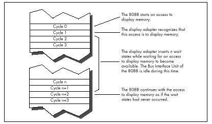
As with DRAM refresh, wait states don’t stop the 8088 completely. The Execution Unit can continue processing while wait states are inserted, so long as the EU doesn’t need to perform a bus access. However, in the PC, wait states most often occur when an instruction accesses a memory operand, so in fact the Execution Unit usually is stopped by wait states. (Instruction fetches rarely wait in an 8088-based PC because system memory is zero-wait-state. AT-class memory systems routinely insert 1 or more wait states, however.)
As it turns out, wait states pose a serious problem in just one area in the PC. While any adapter can insert wait states, in the PC only display adapters do so to the extent that performance is seriously affected.
The Display Adapter Cycle-Eater
Display adapters must serve two masters, and that creates a fundamental performance problem. Master #1 is the circuitry that drives the display screen. This circuitry must constantly read display memory in order to obtain the information used to draw the characters or dots displayed on the screen. Since the screen must be redrawn between 50 and 70 times per second, and since each redraw of the screen can require as many as 36,000 reads of display memory (more in Super VGA modes), master #1 is a demanding master indeed. No matter how demanding master #1 gets, however, its needs must always be met—otherwise the quality of the picture on the screen would suffer.
Master #2 is the CPU, which reads from and writes to display memory in order to manipulate the bytes that the video circuitry reads to form the picture on the screen. Master #2 is less important than master #1, since the CPU affects display quality only indirectly. In other words, if the video circuitry has to wait for display memory accesses, the picture will develop holes, snow, and the like, but if the CPU has to wait for display memory accesses, the program will just run a bit slower—no big deal.
It matters a great deal which master is more important, for while both the CPU and the video circuitry must gain access to display memory, only one of the two masters can read or write display memory at any one time. Potential conflicts are resolved by flat-out guaranteeing the video circuitry however many accesses to display memory it needs, with the CPU waiting for whatever display memory accesses are left over.
It turns out that the 8088 CPU has to do a lot of waiting, for three reasons. First, the video circuitry can take as much as about 90 percent of the available display memory access time, as shown in Figure 4.7, leaving as little as about 10 percent of all display memory accesses for the 8088. (These percentages vary considerably among the many EGA and VGA clones.)
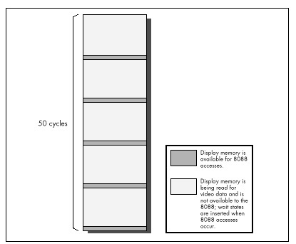
Second, because the displayed dots (or pixels, short for “picture elements”) must be drawn on the screen at a constant speed, many display adapters provide memory accesses only at fixed intervals. As a result, time can be lost while the 8088 synchronizes with the start of the next display adapter memory access, even if the video circuitry isn’t accessing display memory at that time, as shown in Figure 4.8.
Finally, the time it takes a display adapter to complete a memory access is related to the speed of the clock which generates pixels on the screen rather than to the memory access speed of the 8088. Consequently, the time taken for display memory to complete an 8088 read or write access is often longer than the time taken for system memory to complete an access, even if the 8088 lucks into hitting a free display memory access just as it becomes available, again as shown in Figure 4.8. Any or all of the three factors I’ve described can result in wait states, slowing the 8088 and creating the display adapter cycle.
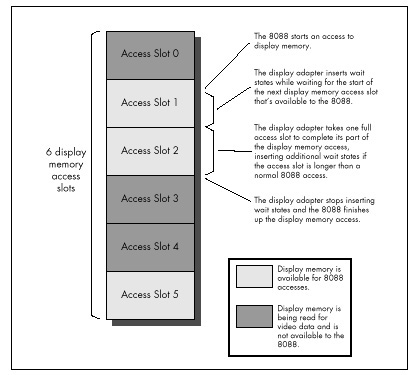
If some of this is Greek to you, don’t worry. The important point is that display memory is not very fast compared to normal system memory. How slow is it? Incredibly slow. Remember how slow IBM’s ill-fated PCjrwas? In case you’ve forgotten, I’ll refresh your memory: The PCjrwas at best only half as fast as the PC. The PCjr had an 8088 running at 4.77 MHz, just like the PC—why do you suppose it was so much slower? I’ll tell you why: All the memory in the PCjr was display memory.
Enough said. All the memory in the PC is not display memory, however, and unless you’re thickheaded enough to put code in display memory, the PC isn’t going to run as slowly as a PCjr. (Putting code or other non-video data in unused areas of display memory sounds like a neat idea—until you consider the effect on instruction prefetching of cutting the 8088’s already-poor memory access performance in half. Running your code from display memory is sort of like running on a hypothetical 8084—an 8086 with a 4-bit bus. Not recommended!) Given that your code and data reside in normal system memory below the 640K mark, how great an impact does the display adapter cycle-eater have on performance?
The answer varies considerably depending on what display adapter and what display mode we’re talking about. The display adapter cycle-eater is worst with the Enhanced Graphics Adapter (EGA) and the original Video Graphics Array (VGA). (Many VGAs, especially newer ones, insert many fewer wait states than IBM’s original VGA. On the other hand, Super VGAs have more bytes of display memory to be accessed in high-resolution mode.) While the Color/Graphics Adapter (CGA), Monochrome Display Adapter (MDA), and Hercules Graphics Card (HGC) all suffer from the display adapter cycle-eater as well, they suffer to a lesser degree. Since the VGA represents the base standard for PC graphics now and for the foreseeable future, and since it is the hardest graphics adapter to wring performance from, we’ll restrict our discussion to the VGA (and its close relative, the EGA) for the remainder of this chapter.
The Impact of the Display Adapter Cycle-Eater
Even on the EGA and VGA, the effect of the display adapter cycle-eater depends on the display mode selected. In text mode, the display adapter cycle-eater is rarely a major factor. It’s not that the cycle-eater isn’t present; however, a mere 4,000 bytes control the entire text mode display, and even with the display adapter cycle-eater it just doesn’t take that long to manipulate 4,000 bytes. Even if the display adapter cycle-eater were to cause the 8088 to take as much as 5µs per display memory access—more than five times normal—it would still take only 4,000x 2x 5µs, or 40 ms, to read and write every byte of display memory. That’s a lot of time as measured in 8088 cycles, but it’s less than the blink of an eye in human time, and video performance only matters in human time. After all, the whole point of drawing graphics is to convey visual information, and if that information can be presented faster than the eye can see, that is by definition fast enough.
That’s not to say that the display adapter cycle-eater can’t matter in text mode. In Chapter 3, I recounted the story of a debate among letter-writers to a magazine about exactly how quickly characters could be written to display memory without causing snow. The writers carefully added up Intel’s instruction cycle times to see how many writes to display memory they could squeeze into a single horizontal retrace interval. (On a CGA, it’s only during the short horizontal retrace interval and the longer vertical retrace interval that display memory can be accessed in 80-column text mode without causing snow.) Of course, now we know that their cardinal sin was to ignore the prefetch queue; even if there were no wait states, their calculations would have been overly optimistic. There are display memory wait states as well, however, so the calculations were not just optimistic but wildly optimistic.
Text mode situations such as the above notwithstanding, where the display adapter cycle-eater really kicks in is in graphics mode, and most especially in the high-resolution graphics modes of the EGA and VGA. The problem here is not that there are necessarily more wait states per access in highgraphics modes (that varies from adapter to adapter and mode to mode). Rather, the problem is simply that are many more bytes of display memory per screen in these modes than in lower-resolution graphics modes and in text modes, so many more display memory accesses—each incurring its share of display memory wait states—are required in order to draw an image of a given size. When accessing the many thousands of bytes used in the high-resolution graphics modes, the cumulative effects of display memory wait states can seriously impact code performance, even as measured in human time.
For example, if we assume the same 5 µs per display memory access for the EGA’s high-resolution graphics mode that we assumed for text mode, it would take 26,000 x 2 x 5 µs, or 260 ms, to scroll the screen once in the EGA’s high-resolution graphics mode, mode 10H. That’s more than one-quarter of a second—noticeable by human standards, an eternity by computer standards.
That sounds pretty serious, but we did make an unfounded assumption
about memory access speed. Let’s get some hard numbers. Listing 4.11
accesses display memory at the 8088’s maximum speed, by way of a
REP MOVSW with display memory as both source and
destination. The code in Listing 4.11 executes in 3.18 µs per access to
display memory—not as long as we had assumed, but a long time
nonetheless.
LISTING 4.11 LST4-11.ASM
; Times speed of memory access to Enhanced Graphics
; Adapter graphics mode display memory at A000:0000.
;
mov ax,0010h
int 10h; select hi-res EGA graphics
; mode 10 hex (AH=0 selects
; BIOS set mode function,
; with AL=mode to select)
;
mov ax,0a000h
mov ds,ax
mov es,ax ;move to & from same segment
sub si,si ;move to & from same offset
mov di,si
mov cx,800h ;move 2K words
cld
call ZTimerOn
rep movsw ;simply read each of the first
; 2K words of the destination segment,
; writing each byte immediately back
; to the same address. No memory
; locations are actually altered; this
; is just to measure memory access
; times
call ZTimerOff
;
mov ax,0003h
int 10h ;return to text modeFor comparison, let’s see how long the same code takes when accessing
normal system RAM instead of display memory. The code in Listing 4.12,
which performs a REP MOVSW from the code segment to the
code segment, executes in 1.39 µs per display memory access. That means
that on average, 1.79 µs (more than 8 cycles!) are lost to the display
adapter cycle-eater on each access. In other words, the display adapter
cycle-eater can more than double the execution time of 8088
code!
LISTING 4.12 LST4-12.ASM
; Times speed of memory access to normal system
; memory.
;
mov ax,ds
mov es,ax ;move to & from same segment
sub si,si ;move to & from same offset
mov di,si
mov cx,800h ;move 2K words
cld
call ZTimerOn
rep movsw ;simply read each of the first
; 2K words of the destination segment,
; writing each byte immediately back
; to the same address. No memory
; locations are actually altered; this
; is just to measure memory access
; times
call ZTimerOffBear in mind that we’re talking about a worst case here; the impact of the display adapter cycle-eater is proportional to the percent of time a given code sequence spends accessing display memory.
REP MOVSinstructions. Scaled and three-dimensional graphics, which spend a great deal of time performing calculations (often using very slow floating-point arithmetic), tend to suffer less.
In addition, code that accesses display memory infrequently tends to suffer only about half of the maximum display memory wait states, because on average such code will access display memory halfway between one available display memory access slot and the next. As a result, code that accesses display memory less intensively than the code in Listing 4.11 will on average lose 4 or 5 rather than 8-plus cycles to the display adapter cycle-eater on each memory access.
Nonetheless, the display adapter cycle-eater always takes its toll on graphics code. Interestingly, that toll becomes much higher on ATs and 80386 machines because while those computers can execute many more instructions per microsecond than can the 8088-based PC, it takes just as long to access display memory on those computers as on the 8088-based PC. Remember, the limited speed of access to a graphics adapter is an inherent characteristic of the adapter, so the fastest computer around can’t access display memory one iota faster than the adapter will allow.
What to Do about the Display Adapter Cycle-Eater?
What can we do about the display adapter cycle-eater? Well, we can minimize display memory accesses whenever possible. In particular, we can try to avoid read/modify/write display memory operations of the sort used to mask individual pixels and clip images. Why? Because read/modify/write operations require two display memory accesses (one read and one write) each time display memory is manipulated. Instead, we should try to use writes of the sort that set all the pixels in a given byte of display memory at once, since such writes don’t require accompanying read accesses. The key here is that only half as many display memory accesses are required to write a byte to display memory as are required to read a byte from display memory, mask part of it off and alter the rest, and write the byte back to display memory. Half as many display memory accesses means half as many display memory wait states.
Along the same line, the display adapter cycle-eater makes the popular exclusive-OR animation technique, which requires paired reads and writes of display memory, less-than-ideal for the PC. Exclusive-OR animation should be avoided in favor of simply writing images to display memory whenever possible.
Another principle for display adapter programming on the 8088 is to perform multiple accesses to display memory very rapidly, in order to make use of as many of the scarce accesses to display memory as possible. This is especially important when many large images need to be drawn quickly, since only by using virtually every available display memory access can many bytes be written to display memory in a short period of time. Repeated string instructions are ideal for making maximum use of display memory accesses; of course, repeated string instructions can only be used on whole bytes, so this is another point in favor of modifying display memory a byte at a time. (On faster processors, however, display memory is so slow that it often pays to do several instructions worth of work between display memory accesses, to take advantage of cycles that would otherwise be wasted on the wait states.)
It would be handy to explore the display adapter cycle-eater issue in depth, with lots of example code and execution timings, but alas, I don’t have the space for that right now. For the time being, all you really need to know about the display adapter cycle-eater is that on the 8088 you can lose more than 8 cycles of execution time on each access to display memory. For intensive access to display memory, the loss really can be as high as 8cycles (and up to 50, 100, or even more on 486s and Pentiums paired with slow VGAs), while for average graphics code the loss is closer to 4 cycles; in either case, the impact on performance is significant. There is only one way to discover just how significant the impact of the display adapter cycle-eater is for any particular graphics code, and that is of course to measure the performance of that code.
Cycle-Eaters: A Summary
We’ve covered a great deal of sophisticated material in this chapter, so don’t feel bad if you haven’t understood everything you’ve read; it will all become clear from further reading, especially once you study, time, and tune code that you have written yourself. What’s really important is that you come away from this chapter understanding that on the 8088:
- The 8-bit bus cycle-eater causes each access to a word-sized operand to be 4 cycles longer than an equivalent access to a byte-sized operand.
- The prefetch queue cycle-eater can cause instruction execution times to be as much as four times longer than the officially documented cycle times.
- The DRAM refresh cycle-eater slows most PC code, with performance reductions ranging as high as 8.33 percent.
- The display adapter cycle-eater typically doubles and can more than triple the length of the standard 4-cycle access to display memory, with intensive display memory access suffering most.
This basic knowledge about cycle-eaters puts you in a good position to understand the results reported by the Zen timer, and that means that you’re well on your way to writing high-performance assembler code.
What Does It All Mean?
There you have it: life under the programming interface. It’s not a particularly pretty picture for the inhabitants of that strange realm where hardware and software meet are little-known cycle-eaters that sap the speed from your unsuspecting code. Still, some of those cycle-eaters can be minimized by keeping instructions short, using the registers, using byte-sized memory operands, and accessing display memory as little as possible. None of the cycle-eaters can be eliminated, and dynamic RAM refresh can scarcely be addressed at all; still, aren’t you better off knowing how fast your code really runs—and why—than you were reading the official execution times and guessing? And while specific cycle-eaters vary in importance on later x86-family processors, with some cycle-eaters vanishing altogether and new ones appearing, the concept that understanding these obscure gremlins is a key to performance remains unchanged, as we’ll see again and again in later chapters.
Chapter 5 – Crossing the Border
Searching Files with Restartable Blocks
We just moved. Those three little words should strike terror into the heart of anyone who owns more than a sleeping bag and a toothbrush. Our last move was the usual zoo—and then some. Because the distance from the old house to the new was only five miles, we used cars to move everything smaller than a washing machine. We have a sizable household—cats, dogs, kids, com, you name it—so the moving process took a number of car trips. A large number—33, to be exact. I personally spent about 15 hours just driving back and forth between the two houses. The move took days to complete.
Never again.
You’re probably wondering two things: What does this have to do with high-performance programming, and why on earth didn’t I rent a truck and get the move over in one or two trips, saving hours of driving? As it happens, the second question answers the first. I didn’t rent a truck because it seemed easier and cheaper to use cars—no big truck to drive, no rentals, spread the work out more manageably, and so on.
It wasn’t easier, and wasn’t even much cheaper. (It costs quite a bit to drive a car 330 miles, to say nothing of the value of 15 hours of my time.) But, at the time, it seemed as though my approach would be easier and cheaper. In fact, I didn’t realize just how much time I had wasted driving back and forth until I sat down to write this chapter.
In Chapter 1, I briefly discussed using restartable blocks. This, you might remember, is the process of handling in chunks data sets too large to fit in memory so that they can be processed just about as fast as if they did fit in memory. The restartable block approach is very fast but is relatively difficult to program.
At the opposite end of the spectrum lies byte-by-byte processing, whereby DOS (or, in less extreme cases, a group of library functions) is allowed to do all the hard work, so that you only have to deal with one byte at a time. Byte-by-byte processing is easy to program but can be extremely slow, due to the vast overhead that results from invoking DOS each time a byte must be processed.
Sound familiar? It should. I moved via the byte-by-byte approach, and the overhead of driving back and forth made for miserable performance. Renting a truck (the restartable block approach) would have required more effort and forethought, but would have paid off handsomely.
And with that, let’s look at a fairly complex application of restartable blocks.
Searching for Text
The application we’re going to examine searches a file for a
specified string. We’ll develop a program that will search the file
specified on the command line for a string (also specified on the
comline), then report whether the string was found or not. (Because the
searched-for string is obtained via argv, it can’t contain
any whitespace characters.)
This is a very limited subset of what search utilities such as grep can do, and isn’t really intended to be a generally useful application; the purpose is to provide insight into restartable blocks in particular and optimization in general in the course of developing a search engine. That search engine will, however, be easy to plug into any program, and there’s nothing preventing you from using it in a more fruitful context, like searching through a user-selectable file set.
The first point to address in designing our program involves the appropriate text-search approach to use. Literally dozens of workable ways exist to search a file. We can immediately discard all approaches that involve reading any byte of the file more than once, because disk access time is orders of magnitude slower than any data handling performed by our own code. Based on our experience in Chapter 1, we can also discard all approaches that get bytes either one at a time or in small sets from DOS. We want to read big “buffers-full” of bytes at a pop from the searched file, and the bigger the buffer the better—in order to minimize DOS’s overhead. A good rough cut is a buffer that will be between 16K and 64K, depending on the exact search approach, 64K being the maximum size because near pointers make for superior performance.
So we know we want to work with a large buffer, filling it as infrequently as possible. Now we have to figure out how to search through a file by loading it into that large buffer in chunks. To accomplish this, we have to know how we want to do our searching, and that’s not immediately obvious. Where do we begin?
Well, it might be instructive to consider how we would search if our search involved only one buffer, already resident in memory. In other words, suppose we don’t have to bother with file handling at all, and further suppose that we don’t have to deal with searching through multiple blocks. After all, that’s a good description of the all-important inner loop of our searching program, where the program will spend virtually all of its time (aside from the unavoidable disk access overhead).
Avoiding the String Trap
The easiest approach would be to use a C/C++ library function. The
closest match to what we need is strstr(), which searches
one string for the first occurrence of a second string. However, while
strstr() would work, it isn’t ideal for our purposes. The
problem is this: Where we want to search a fixed-length buffer for the
first occurrence of a string, strstr() searches a
string for the first occurrence of another string.
We could put a zero byte at the end of our buffer to allow
strstr() to work, but why bother? The strstr()
function must spend time either checking for the end of the string being
searched or determining the length of that string—wasted effort given
that we already know exactly how long our search buffer is. Even if a
given strstr() implementation is well-written, its
performance will suffer, at least for our application, from unnecessary
overhead.
Brute-Force Techniques
Given that no C/C++ library function meets our needs precisely, an
obvious alternative approach is the brute-force technique that uses
memcmp() to compare every potential matching
location in the buffer to the string we’re searching for, as illustrated
in Figure 5.1.
By the way, we could, of course, use our own code, working with
pointers in a loop, to perform the comparison in place of
memcmp(). But memcmp() will almost certainly
use the very fast REPZ CMPS instruction. However, never
assume! It wouldn’t hurt to use a debugger to check out the actual
machine-code implementation of memcmp() from your compiler.
If necessary, you could always write your own assembly language
implementation of memcmp().
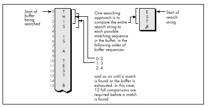
Invoking memcmp() for each potential match location
works, but entails considerable overhead. Each comparison requires that
parameters be pushed and that a call to and return from
memcmp() be performed, along with a pass through the
comparison loop. Surely there’s a better way!
Indeed there is. We can eliminate most calls to memcmp()
by performing a simple test on each potential match location that will
reject most such locations right off the bat. We’ll just check whether
the first character of the potentially matching buffer location matches
the first character of the string we’re searching for. We could make
this check by using a pointer in a loop to scan the buffer for the next
match for the first character, stopping to check for a match with the
rest of the string only when the first character matches, as
shown in Figure 5.2.
Using memchr()
There’s yet a better way to implement this approach, however. Use the
memchr() function, which does nothing more or less than
find the next occurrence of a specified character in a fixed-length
buffer (presumably by using the extremely efficient
REPNZ SCASB instruction, although again it wouldn’t hurt to
check). By using memchr() to scan for potential matches
that can then be fully tested with memcmp(), we can build a
highly efficient search engine that takes good advantage of the
information we have about the buffer being searched and the string we’re
searching for. Our engine also relies heavily on repeated string
instructions, assuming that the memchr() and
memcmp() library functions are properly coded.
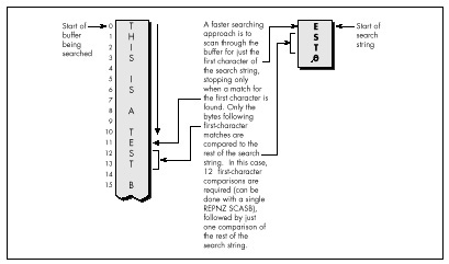
We’re going to go with the this approach in our file-searching program; the only trick lies in deciding how to integrate this approach with restartable blocks in order to search through files larger than our buffer. This certainly isn’t the fastest-possible searching algorithm; as one example, the Boyer-Moore algorithm, which cleverly eliminates many buffer locations as potential matches in the process of checking preceding locations, can be considerably faster. However, the Boyer-Moore algorithm is quite complex to understand and implement, and would distract us from our main focus, restartable blocks, so we’ll save it for a later chapter (Chapter 14, to be precise). Besides, I suspect you’ll find the approach we’ll use to be fast enough for most purposes.
Now that we’ve selected a searching approach, let’s integrate it with file handling and searching through multiple blocks. In other words, let’s make it restartable.
Making a Search Restartable
As it happens, there’s no great trick to putting the pieces of this
search program together. Basically, we’ll read in a buffer of data
(we’ll work with 16K at a time to avoid signed overflow problems with
integers), search it for a match with the
memchr()/memcmp() engine described, and exit
with a “string found” response if the desired string is found.
Otherwise, we’ll load in another buffer full of data from the file, search it, and so on. The only trick lies in handling potentially matching sequences in the file that start in one buffer and end in the next—that is, sequences that span buffers. We’ll handle this by copying the unchecked bytes at the end of one buffer to the start of the next and reading that many fewer bytes the next time we fill the buffer.
The exact number of bytes to be copied from the end of one buffer to the start of the next is the length of the searched-for string minus 1, since that’s how many bytes at the end of the buffer can’t be checked as possible matches (because the check would run off the end of the buffer).
That’s really all there is to it. Listing 5.1 shows the
file-searching program. As you can see, it’s not particularly complex,
although a few fairly opaque lines of code are required to handle
merging the end of one block with the start of the next. The code that
searches a single block—the function SearchForString()—is
simple and compact (as it should be, given that it’s by far the most
heavily-executed code in the listing).
Listing 5.1 nicely illustrates the core concept of restartable blocks: Organize your program so that you can do your processing within each block as fast as you could if there were only one block—which is to say at top speed—and make your blocks as large as possible in order to minimize the overhead associated with going from one block to the next.
LISTING 5.1 SEARCH.C
/* Program to search the file specified by the first command-line
* argument for the string specified by the second command-line
* argument. Performs the search by reading and searching blocks
* of size BLOCK_SIZE. */
#include <stdio.h>
#include <fcntl.h>
#include <string.h>
#include <alloc.h> /* alloc.h for Borland compilers,
malloc.h for Microsoft compilers */
#define BLOCK_SIZE 0x4000 /* we'll process the file in 16K blocks */
/* Searches the specified number of sequences in the specified
buffer for matches to SearchString of SearchStringLength. Note
that the calling code should already have shortened SearchLength
if necessary to compensate for the distance from the end of the
buffer to the last possible start of a matching sequence in the
buffer.
*/
int SearchForString(unsigned char *Buffer, int SearchLength,
unsigned char *SearchString, int SearchStringLength)
{
unsigned char *PotentialMatch;
/* Search so long as there are potential-match locations
remaining */
while ( SearchLength ) {
/* See if the first character of SearchString can be found */
if ( (PotentialMatch =
memchr(Buffer, *SearchString, SearchLength)) == NULL ) {
break; /* No matches in this buffer */
}
/* The first character matches; see if the rest of the string
also matches */
if ( SearchStringLength == 1 ) {
return(1); /* That one matching character was the whole
search string, so we've got a match */
}
else {
/* Check whether the remaining characters match */
if ( !memcmp(PotentialMatch + 1, SearchString + 1,
SearchStringLength - 1) ) {
return(1); /* We've got a match */
}
}
/* The string doesn't match; keep going by pointing past the
potential match location we just rejected */
SearchLength -= PotentialMatch - Buffer + 1;
Buffer = PotentialMatch + 1;
}
return(0); /* No match found */
}
main(int argc, char *argv[]) {
int Done; /* Indicates whether search is done */
int Handle; /* Handle of file being searched */
int WorkingLength; /* Length of current block */
int SearchStringLength; /* Length of string to search for */
int BlockSearchLength; /* Length to search in current block */
int Found; /* Indicates final search completion
status */
int NextLoadCount; /* # of bytes to read into next block,
accounting for bytes copied from the
last block */
unsigned char *WorkingBlock; /* Block storage buffer */
unsigned char *SearchString; /* Pointer to the string to search for */
unsigned char *NextLoadPtr; /* Offset at which to start loading
the next block, accounting for
bytes copied from the last block */
/* Check for the proper number of arguments */
if ( argc != 3 ) {
printf("usage: search filename search-string\n");
exit(1);
}
/* Try to open the file to be searched */
if ( (Handle = open(argv[1], O_RDONLY | O_BINARY)) == -1 ) {
printf("Can't open file: %s\n", argv[1]);
exit(1);
}
/* Calculate the length of text to search for */
SearchString = argv[2];
SearchStringLength = strlen(SearchString);
/* Try to get memory in which to buffer the data */
if ( (WorkingBlock = malloc(BLOCK_SIZE)) == NULL ) {
printf("Can't get enough memory\n");
exit(1);
}
/* Load the first block at the start of the buffer, and try to
fill the entire buffer */
NextLoadPtr = WorkingBlock;
NextLoadCount = BLOCK_SIZE;
Done = 0; /* Not done with search yet */
Found = 0; /* Assume we won't find a match */
/* Search the file in BLOCK_SIZE chunks */
do {
/* Read in however many bytes are needed to fill out the block
(accounting for bytes copied over from the last block), or
the rest of the bytes in the file, whichever is less */
if ( (WorkingLength = read(Handle, NextLoadPtr,
NextLoadCount)) == -1 ) {
printf("Error reading file %s\n", argv[1]);
exit(1);
}
/* If we didn't read all the bytes we requested, we're done
after this block, whether we find a match or not */
if ( WorkingLength != NextLoadCount ) {
Done = 1;
}
/* Account for any bytes we copied from the end of the last
block in the total length of this block */
WorkingLength += NextLoadPtr - WorkingBlock;
/* Calculate the number of bytes in this block that could
possibly be the start of a matching sequence that lies
entirely in this block (sequences that run off the end of
the block will be transferred to the next block and found
when that block is searched)
*/
if ( (BlockSearchLength =
WorkingLength - SearchStringLength + 1) <= 0 ) {
Done = 1; /* Too few characters in this block for
there to be any possible matches, so this
is the final block and we're done without
finding a match
*/
}
else {
/* Search this block */
if ( SearchForString(WorkingBlock, BlockSearchLength,
SearchString, SearchStringLength) ) {
Found = 1; /* We've found a match */
Done = 1;
}
else {
/* Copy any bytes from the end of the block that start
potentially-matching sequences that would run off
the end of the block over to the next block */
if ( SearchStringLength > 1 ) {
memcpy(WorkingBlock,
WorkingBlock+BLOCK_SIZE - SearchStringLength + 1,
SearchStringLength - 1);
}
/* Set up to load the next bytes from the file after the
bytes copied from the end of the current block */
NextLoadPtr = WorkingBlock + SearchStringLength - 1;
NextLoadCount = BLOCK_SIZE - SearchStringLength + 1;
}
}
} while ( !Done );
/* Report the results */
if ( Found ) {
printf("String found\n");
} else {
printf("String not found\n");
}
exit(Found); /* Return the found/not found status as the
DOS errorlevel */
}Interpreting Where the Cycles Go
To boost the overall performance of Listing 5.1, I would normally
convert SearchForString() to assembly language at this
point. However, I’m not going to do that, and the reason is as important
a lesson as any discussion of optimized assembly code is likely to be.
Take a moment to examine some interesting performance aspects of the C
implementation, and all should become much clearer.
As you’ll recall from Chapter 1, one of the important rules for optimization involves knowing when optimization is worth bothering with at all. Another rule involves understanding where most of a program’s execution time is going. That’s more true for Listing 5.1 than you might think.
When Listing 5.1 is run on a 1 MB assembly source file, it takes
about three seconds to find the string “xxxend” (which is at the end of
the file) on a 20 MHz 386 machine, with the entire file in a disk cache.
If BLOCK_SIZE is trimmed from 16K to 4K, execution time
does not increase perceptibly! At 2K, the program slows slightly;
it’s not until the block size shrinks to 64 bytes that execution time
becomes approximately double that of the 16K buffer.
So the first thing we’ve discovered is that, while bigger blocks do
make for the best performance, the increment in performance may not be
very large, and might not justify the extra memory required for those
larger blocks. Our next discovery is that, even though we read the file
in large chunks, most of the execution time of Listing 5.1 is
nonetheless spent in executing the read() function.
When I replaced the read() function call in Listing 5.1
with code that simply fools the program into thinking that a 1 MB file
is being read, the program ran almost instantaneously—in less than 1/2
second, even when the searched-for string wasn’t anywhere to be found.
By contrast, Listing 5.1 requires three seconds to run even when
searching for a single character that isn’t found anywhere in the file,
the case in which a single call to memchr() (and thus a
single REPNZ SCASB) can eliminate an entire block at a
time.
All in all, the time required for DOS disk access calls is taking up
at least 80 percent of execution time, and search time is less than 20
percent of overall execution time. In fact, search time is probably a
good deal less than 20 percent of the total, given that the overhead of
loading the program, running through the C startup code, opening the
file, executing printf(), and exiting the program and
returning to the DOS shell are also included in my timings. Given which,
it should be apparent why converting to assembly language isn’t worth
the trouble—the best we could do by speeding up the search is a 10
percent or so improvement, and that would require more than doubling the
performance of code that already uses repeated string instructions to do
most of the work.
Not likely.
Knowing When Assembly Is Pointless
So that’s why we’re not going to go to assembly language in this example—which is not to say it would never be worth converting the search engine in Listing 5.1 to assembly.
If, for example, your application will typically search buffers in
which the first character of the search string occurs frequently as
might be the case when searching a text buffer for a string starting
with the space character an assembly implementation might be several
times faster. Why? Because assembly code can switch from
REPNZ SCASB to match the first character to
REPZ CMPS to check the remaining characters in just a few
instructions.
In contrast, Listing 5.1 must return from memchr(), set
up parameters, and call memcmp() in order to do the same
thing. Likewise, assembly can switch back to REPNZ SCASB
after a non-match much more quickly than Listing 5.1. The switching
overhead is high; when searching a file completely filled with the
character z for the string “zy,” Listing 5.1 takes almost 1/2 minute, or
nearly an order of magnitude longer than when searching a file filled
with normal text.
It might also be worth converting the search engine to assembly for searches performed entirely in memory; with the overhead of file access eliminated, improvements in search-engine performance would translate directly into significantly faster overall performance. One such application that would have much the same structure as Listing 5.1 would be searching through expanded memory buffers, and another would be searching through huge (segment-spanning) buffers.
And so we find, as we so often will, that optimization is definitely not a cut-and-dried matter, and that there is no such thing as a single “best” approach.
By the way, don’t think that just because very large block sizes don’t much improve performance, it wasn’t worth using restartable blocks in Listing 5.1. Listing 5.1 runs more than three times more slowly with a block size of 32 bytes than with a block size of 4K, and any byte-by-byte approach would surely be slower still, due to the overhead of repeated calls to DOS and/or the C stream I/O library.
Restartable blocks do minimize the overhead of DOS file-access calls in Listing 5.1; it’s just that there’s no way to reduce that overhead to the point where it becomes worth attempting to further improve the performance of our relatively efficient search engine. Although the search engine is by no means fully optimized, it’s nonetheless as fast as there’s any reason for it to be, given the balance of performance among the components of this program.
Always Look Where Execution Is Going
I’ve explained two important lessons: Know when it’s worth optimizing further, and use restartable blocks to process large data sets as a series of blocks, with each block handled at high speed. The first lesson is less obvious than it seems.
When I set out to write this chapter, I fully intended to write an
assembly language version of Listing 5.1, and I expected the assembly
version to be much faster. When I actually looked at where execution
time was going (which I did by modifying the program to remove the calls
to the read() function, but a code profiler could be used
to do the same thing much more easily), I found that the best code in
the world wouldn’t make much difference.
As for restartable blocks: Here we tackled a considerably more complex application of restartable blocks than we did in Chapter 1—which turned out not to be so difficult after all. Don’t let irregularities in the programming tasks you tackle, such as strings that span blocks, fluster you into settling for easy, general—and slow—solutions. Focus on making the inner loop—the code that handles each block—as efficient as possible, then structure the rest of your code to support the inner loop.
Programming with restartable blocks isn’t easy, but when speed is an issue, using restartable blocks in the right places more than pays for itself with greatly improved performance. And when speed is not an issue, of course, or in code that’s not time-critical, you wouldn’t dream of wasting your time on optimization.
Would you?
Chapter 6 – Looking Past Face Value
How Machine Instructions May Do More Than You Think
I first met Jeff Duntemann at an authors’ dinner hosted by PC Tech Journal at Fall Comdex, back in 1985. Jeff was already reasonably well-known as a computer editor and writer, although not as famous as Complete Turbo Pascal, editions 1 through 672 (or thereabouts), TURBO TECHNIX, and PC TECHNIQUES would soon make him. I was fortunate enough to be seated next to Jeff at the dinner table, and, not surprisingly, our often animated conversation revolved around computers, computer writing, and more computers (not necessarily in that order).
Although I was making a living at computer work and enjoying it at the time, I nonetheless harbored vague ambitions of being a science-fiction writer when I grew up. (I have since realized that this hardly puts me in elite company, especially in the computer world, where it seems that every other person has told me they plan to write science fiction “someday.” Given that probably fewer than 500—I’m guessing here—original science fiction and fantasy short stories, and perhaps a few more novels than that, are published each year in this country, I see a few mid-life crises coming.)
At any rate, I had accumulated a small collection of rejection slips, and fancied myself something of an old hand in the field. At the end of the dinner, as the other writers complained half-seriously about how little they were paid for writing for Tech Journal, I leaned over to Jeff and whispered, “You know, the pay isn’t so bad here. You should see what they pay for science fiction—even to the guys who win awards!”
To which Jeff replied, “I know. I’ve been nominated for two Hugos.”
Oh.
Had I known I was seated next to a real, live science-fiction writer—an award-nominated writer, by God!—I would have pumped him for all I was worth, but the possibility had never occurred to me. I was at a dinner put on by a computer magazine, seated next to an editor who had just finished a book about Turbo Pascal, and, gosh, it was obvious that the appropriate topic was computers.
For once, the moral is not “don’t judge a book by its cover.” Jeff is in fact what he appeared to be at face value: a computer writer and editor. However, he is more, too; face value wasn’t full value. You’ll similarly find that face value isn’t always full value in computer programming, and especially so when working in assembly language, where many instructions have talents above and beyond their obvious abilities.
On the other hand, there are also a number of instructions, such as
LOOP, that are designed to perform specific functions but
aren’t always the best instructions for those functions. So don’t judge
a book by its cover, either.
Assembly language for the x86 family isn’t like any other language (for which we should, without hesitation, offer our profuse thanks). Assembly language reflects the design of the processor rather than the way we think, so it’s full of multiple instructions that perform similar functions, instructions with odd and often confusing side effects, and endless ways to string together different instructions to do much the same things, often with seemingly minuscule differences that can turn out to be surprisingly important.
To produce the best code, you must decide precisely what you need to accomplish, then put together the sequence of instructions that accomplishes that end most efficiently, regardless of what the instructions are usually used for. That’s why optimization for the PC is an art, and it’s why the best assembly language for the x86 family will almost always handily outperform compiled code. With that in mind, let’s look past face value—and while we’re at it, I’ll toss in a few examples of not judging a book by its cover.
The point to all this: You must come to regard the x86 family
instructions for what they do, not what you’re used to thinking they do.
Yes, SHL shifts a pattern left—but a look-up table can do
the same thing, and can often do it faster. ADD can indeed
add two operands, but it can’t put the result in a third register;
LEA can. The instruction set is your raw material for
writing high-performance code. By limiting yourself to thinking only in
certain well-established ways about the various instructions, you’re
putting yourself at a substantial disadvantage every time you sit down
to program.
In short, the x86 family can do much more than you think—if you’ll use everything it has to offer. Give it a shot!
Memory Addressing and Arithmetic
Years ago, I saw a clip on the David Letterman show in which Letterman walked into a store by the name of “Just Lamps” and asked, “So what do you sell here?”
“Lamps,” he was told. “Just lamps. Can’t you read?”
“Lamps,” he said. “I see. And what else?”
From that bit of sublime idiocy we can learn much about divining the full value of an instruction. To wit:
Quick, what do the x86’s memory addressing modes do?
“Calculate memory addresses,” you no doubt replied. And you’re right, of course. But what else do they do?
They perform arithmetic, that’s what they do, and that’s a distinctly different and often useful perspective on memory address calculations.
For example, suppose you have an array base address in BX and an index into the array in SI. You could add the two registers together to address memory, like this:
add bx,si
mov al,[bx]Or you could let the processor do the arithmetic for you in a single instruction:
mov al,[bx+si]The two approaches are functionally interchangeable but not
equivalent from a performance standpoint, and which is better depends on
the particular context. If it’s a one-shot memory access, it’s best to
let the processor perform the addition; it’s generally faster at doing
this than a separate ADD instruction would be. If it’s a
memory access within a loop, however, it’s advantageous on the 8088 CPU
to perform the addition outside the loop, if possible, reducing
effective address calculation time inside the loop, as in the
following:
add bx,si
LoopTop:
mov al,[bx]
inc bx
loop LoopTopHere, MOV AL,[BX] is two cycles faster than
MOV AL,[BX+SI].
On a 286 or 386, however, the balance shifts.
MOV AL,[BX+SI] takes no longer than
MOV AL,[BX] on these processors because effective address
calculations generally take no extra time at all. (According to the MASM
manual, one extra clock is required if three memory addressing
components, as in MOV AL,[BX+SI+1], are used. I have not
been able to confirm this from Intel publications, but then I haven’t
looked all that hard.) If you’re optimizing for the 286 or 386, then,
you can take advantage of the processor’s ability to perform arithmetic
as part of memory address calculations without taking a performance
hit.
The 486 is an odd case, in which the use of an index register or the use of a base register that’s the destination of the previous instruction may slow things down, so it is generally but not always better to perform the addition outside the loop on the 486. All memory addressing calculations are free on the Pentium, however. I’ll discuss 486 performance issues in Chapters 12 and 13, and the Pentium in Chapters 19 through 21.
Math via Memory Addressing
You’re probably not particularly wowed to hear that you can use addressing modes to perform memory addressing arithmetic that would otherwise have to be performed with separate arithmetic instructions. You may, however, be a tad more interested to hear that you can also use addressing modes to perform arithmetic that has nothing to do with memory addressing, and with a couple of advantages over arithmetic instructions, at that.
How?
With LEA, the only instruction that performs memory
addressing calculations but doesn’t actually address memory.
LEA accepts a standard memory addressing operand, but does
nothing more than store the calculated memory offset in the specified
register, which may be any general-purpose register. The operation of
LEA is illustrated in Figure 6.1, which also shows the
operation of register-to-register ADD, for comparison.
What does that give us? Two things that ADD doesn’t
provide: the ability to perform addition with either two or three
operands, and the ability to store the result in any register,
not just in one of the source operands.
Imagine that we want to add BX to DI, add two to the result, and store the result in AX. The obvious solution is this:
mov ax,bx
add ax,di
add ax,2(It would be more compact to increment AX twice than to add two to it, and would probably be faster on an 8088, but that’s not what we’re after at the moment.) An elegant alternative solution is simply:
lea ax,[bx+di+2]Likewise, either of the following would copy SI plus two to DI
mov di,si
add di,2or:
lea di,[si+2]Mind you, the only components LEA can add are BX or BP,
SI or DI, and a constant displacement, so it’s not going to replace
ADD most of the time. Also, LEA is
considerably slower than ADD on an 8088, although it is
just as fast as ADD on a 286 or 386 when fewer than three
memory addressing components are used. LEA is 1 cycle
slower than ADD on a 486 if the sum of two registers is
used to point to memory, but no slower than ADD on a
Pentium. On both a 486 and Pentium, LEA can also be slowed
down by addressing interlocks.
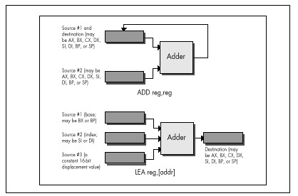
The Wonders of LEA on the 386
LEA really comes into its own as a “super-ADD”
instruction on the 386, 486, and Pentium, where it can take advantage of
the enhanced memory addressing modes of those processors. (The 486 and
Pentium offer the same modes as the 386, so I’ll refer only to the 386
from now on.) The 386 can do two very interesting things: It can use
any 32-bit register (EAX, EBX, and so on) as the memory
addressing base register and/or the memory addressing index register,
and it can multiply any 32-bit register used as an index by two, four,
or eight in the process of calculating a memory address, as shown in
Figure 6.2. Let’s see what that’s good for.
Well, the obvious advantage is that any two 32-bit registers, or any
32-bit register and any constant, or any two 32-bit registers and any
constant, can be added together, with the result stored in any register.
This makes the 32-bit LEA much more generally useful than
the standard 16-bit LEA in the role of an ADD
with an independent destination.
![Figure 6.2 Operation of the 32-bit LEA reg,[Addr].](images/06-02.jpg)
But what else can LEA do on a 386, besides add?
It can multiply any register used as an index. LEA can
multiply only by the power-of-two values 2, 4, or 8, but that’s useful
more often than you might imagine, especially when dealing with pointers
into tables. Besides, multiplying by 2, 4, or 8 amounts to a left shift
of 1, 2, or 3 bits, so we can now add up to two 32-bit registers and a
constant, and shift (or multiply) one of the registers to some
extent—all with a single instruction. For example,
lea edi,TableBase[ecx+edx*4]replaces all this
mov edi,edx
shl edi,2
add edi,ecx
add edi,offset TableBasewhen pointing to an entry in a doubly indexed table.
Multiplication with LEA Using Non-Powers of Two
Are you impressed yet with all that LEA can do on the
386? Believe it or not, one more feature still awaits us.
LEA can actually perform a fast multiply of a 32-bit
register by some values other than powers of two. You see, the
same 32-bit register can be both base and index on the 386, and can be
scaled as the index while being used unchanged as the base. That means
that you can, for example, multiply EBX by 5 with:
lea ebx,[ebx+ebx*4]Without LEA and scaling, multiplication of EBX by 5
would require either a relatively slow MUL, along with a
set-up instruction or two, or three separate instructions along the
lines of the following
mov edx,ebx
shl ebx,2
add ebx,edxand would in either case require the destruction of the contents of another register.
Multiplying a 32-bit value by a non-power-of-two multiplier in just 2 cycles is a pretty neat trick, even though it works only on a 386 or 486.
LEAcan multiply a register by on a 386 or 486 is: 2, 3, 4, 5, 8, and 9. That list doesn’t include every multiplier you might want, but it covers some commonly used ones, and the performance is hard to beat.
I’d like to extend my thanks to Duane Strong of Metagraphics for his
help in brainstorming uses for the 386 version of LEA and
for pointing out the complications of 486 instruction timings.
Chapter 7 – Local Optimization
Optimizing Halfway between Algorithms and Cycle Counting
You might not think it, but there’s much to learn about performance programming from the Great Buffalo Sauna Fiasco. To wit:
The scene is Buffalo, New York, in the dead of winter, with the snow piled several feet deep. Four college students, living in typical student housing, are frozen to the bone. The third floor of their house, uninsulated and so cold that it’s uninhabitable, has an ancient bathroom. One fabulously cold day, inspiration strikes:
“Hey—we could make that bathroom into a sauna!”
Pandemonium ensues. Someone rushes out and buys a gas heater, and at considerable risk to life and limb hooks it up to an abandoned but still live gas pipe that once fed a stove on the third floor. Someone else gets sheets of plastic and lines the walls of the bathroom to keep the moisture in, and yet another student gets a bucket full of rocks. The remaining chap brings up some old wooden chairs and sets them up to make benches along the sides of the bathroom. Voila—instant sauna!
They crank up the gas heater, put the bucket of rocks in front of it, close the door, take off their clothes, and sit down to steam themselves. Mind you, it’s not yet 50 degrees Fahrenheit in this room, but the gas heater is roaring. Surely warmer times await.
Indeed they do. The temperature climbs to 55 degrees, then 60, then 63, then 65, and finally creeps up to 68 degrees.
And there it stops.
68 degrees is warm for an uninsulated third floor in Buffalo in the dead of winter. Damn warm. It is not, however, particularly warm for a sauna. Eventually someone acknowledges the obvious and allows that it might have been a stupid idea after all, and everyone agrees, and they shut off the heater and leave, each no doubt offering silent thanks that they had gotten out of this without any incidents requiring major surgery.
And so we see that the best idea in the world can fail for lack of either proper design or adequate horsepower. The primary cause of the Great Buffalo Sauna Fiasco was a lack of horsepower; the gas heater was flat-out undersized. This is analogous to trying to write programs that incorporate features like bitmapped text and searching of multisegment buffers without using high-performance assembly language. Any PC language can perform just about any function you can think of—eventually. That heater would eventually have heated the room to 110 degrees, too—along about the first of June or so.
The Great Buffalo Sauna Fiasco also suffered from fundamental design flaws. A more powerful heater would indeed have made the room hotter—and might well have burned the house down in the process. Likewise, proper algorithm selection and good design are fundamental to performance. The extra horsepower a superb assembly language implementation gives a program is worth bothering with only in the context of a good design.
So, drawing fortitude from the knowledge that our quest is a pure and worthy one, let’s resume our exploration of assembly language instructions with hidden talents and instructions with well-known talents that are less than they appear to be. In the process, we’ll come to see that there is another, very important optimization level between the algorithm/design level and the cycle-counting/individual instruction level. I’ll call this middle level local optimization; it involves focusing on optimizing sequences of instructions rather than individual instructions, all with an eye to implementing designs as efficiently as possible given the capabilities of the x86 family instruction set.
And yes, in case you’re wondering, the above story is indeed true. Was I there? Let me put it this way: If I were, I’d never admit it!
When LOOP Is a Bad Idea
Let’s examine first an instruction that is less than it appears to
be: LOOP. There’s no mystery about what LOOP
does; it decrements CX and branches if CX doesn’t decrement to zero.
It’s so beautifully suited to the task of counting down loops that any
experienced x86 programmer instinctively stuffs the loop count in CX and
reaches for LOOP when setting up a loop. That’s
fine—LOOP does, of course, work as advertised—but there is
one problem:
LOOPis slower thanDEC CXfollowed byJNZ. (Granted,DEC CX/JNZisn’t precisely equivalent toLOOP, becauseDECalters the flags and LOOP doesn’t, but in most situations they’re comparable.)
How can this be? Don’t ask me, ask Intel. On the 8088 and 80286,
LOOP is indeed faster than DEC CX/JNZ by a
cycle, and LOOP is generally a little faster still because
it’s a byte shorter and so can be fetched faster. On the 386, however,
things change; LOOP is two cycles slower than
DEC/JNZ and the fetch time for one extra byte on even an
uncached 386 generally isn’t significant. (Remember that the 386 fetches
four instruction bytes at a pop.) LOOP is three cycles
slower than DEC/JNZ on the 486, and the 486 executes
instructions in so few cycles that those three cycles mean that
DEC/JNZ is nearly twice as fast as
LOOP. Then, too, unlike LOOP, DEC doesn’t
require that CX be used, so the DEC/JNZ
solution is both faster and more flexible on the 386 and 486, and on the
Pentium as well. (By the way, all this is not just theory; I’ve timed
the relative performances of LOOP and
DEC CX/JNZ on a cached 386, and LOOP really is slower.)
LOOP’s relativeJCXZ, which branches if and only if CX is zero.JCXZis faster thanAND CX,CX/JZon the 8088 and 80286, and equivalent on the 80386—but is about twice as slow on the 486!
By the way, don’t fall victim to the lures of JCXZ and
do something like this:
and cx,ofh ;Isolate the desired field
jcxz SkipLoop ;If field is 0, don't botherThe AND instruction has already set the Zero flag, so
this
and cx,0fh ;Isolate the desired field
jz SkipLoop ;If field is 0, don't botherwill do just fine and is faster on all processors. Use
JCXZ only when the Zero flag isn’t already set to reflect
the status of CX.
The Lessons of LOOP and JCXZ
What can we learn from LOOP and JCXZ?
First, that a single instruction that is intended to do a complex task
is not necessarily faster than several instructions that together do the
same thing. Second, that the relative merits of instructions and
optimization rules vary to a surprisingly large degree across the x86
family.
In particular, if you’re going to write 386 protected mode code,
which will run only on the 386, 486, and Pentium, you’d be well advised
to rethink your use of the more esoteric members of the x86 instruction
set. LOOP, JCXZ, the various accumulator-specific
instructions, and even the string instructions in many circumstances no
longer offer the advantages they did on the 8088. Sometimes they’re just
not any faster than more general instructions, so they’re not worth
going out of your way to use; sometimes, as with LOOP,
they’re actually slower, and you’d do well to avoid them altogether in
the 386/486 world. Reviewing the instruction cycle times in the MASM or
TASM manuals, or looking over the cycle times in Intel’s literature, is
a good place to start; published cycle times are closer to actual
execution times on the 386 and 486 than on the 8088, and are reasonably
reliable indicators of the relative performance levels of x86
instructions.
Avoiding LOOPS of Any Stripe
Cycle counting and directly substituting instructions
(DEC CX/JNZ for LOOP, for example) are
techniques that belong at the lowest level of optimization. It’s an
important level, but it’s fairly mechanical; once you’ve learned the
capabilities and relative performance levels of the various
instructions, you should be able to select the best instructions fairly
easily. What’s more, this is a task at which compilers excel. What I’m
saying is that you shouldn’t get too caught up in counting cycles
because that’s a small (albeit important) part of the optimization
picture, and not the area in which your greatest advantage lies.
Local Optimization
One level at which assembly language programming pays off handsomely is that of local optimization; that is, selecting the best sequence of instructions for a task. The key to local optimization is viewing the 80x86 instruction set as a set of building blocks, each with unique characteristics. Your job is to sequence those blocks so that they perform well. It doesn’t matter what the instructions are intended to do or what their names are; all that matters is what they do.
Our discussion of LOOP versus DEC/JNZ is an
excellent example of optimization by cycle counting. It’s worth knowing,
but once you’ve learned it, you just routinely use DEC/JNZ
at the bottom of loops in 386/486-specific code, and that’s that.
Besides, you’ll save at most a few cycles each time, and while that
helps a little, it’s not going to make all that much
difference.
Now let’s step back for a moment, and with no preconceptions consider
what the x86 instruction set can do for us. The bulk of the time with
both LOOP and DEC/JNZ is taken up by
branching, which just happens to be one of the slowest aspects of every
processor in the x86 family, and the rest is taken up by decrementing
the count register and checking whether it’s zero. There may be ways to
perform those tasks a little faster by selecting different instructions,
but they can get only so fast, and branching can’t even get all that
fast.
Consider Listing 7.1, which searches a buffer until either the
specified byte is found, a zero byte is found, or the specified number
of characters have been checked. Such a function would be useful for
scanning up to a maximum number of characters in a zero-terminated
buffer. Listing 7.1, which uses LOOP in the main loop,
performs a search of the sample string for a period (‘.’) in 170 µs on a
20 MHz cached 386.
When the LOOP in Listing 7.1 is replaced with
DEC CX/JNZ, performance improves to 168 µs, less than 2
percent faster than Listing 7.1. Actually, instruction fetching,
instruction alignment, cache characteristics, or something similar is
affecting these results; I’d expect a slightly larger improvement—around
7 percent—but that’s the most that counting cycles could buy us in this
case. (All right, already; LOOPNZ could be used at the
bottom of the loop, and other optimizations are surely possible, but all
that won’t add up to anywhere near the benefits we’re about to see from
local optimization, and that’s the whole point.)
LISTING 7.1 L7-1.ASM
; Program to illustrate searching through a buffer of a specified
; length until either a specified byte or a zero byte is
; encountered.
; A standard loop terminated with LOOP is used.
.model small
.stack 100h
.data
; Sample string to search through.
SampleString label byte
db 'This is a sample string of a long enough length '
db 'so that raw searching speed can outweigh any '
db 'extra set-up time that may be required.',0
SAMPLE_STRING_LENGTH equ $-SampleString
; User prompt.
Prompt db 'Enter character to search for:$'
; Result status messages.
ByteFoundMsg db 0dh,0ah
db 'Specified byte found.',0dh,0ah,'$'
ZeroByteFoundMsg db 0dh, 0ah
db 'Zero byte encountered.',0dh,0ah,'$'
NoByteFoundMsg db 0dh,0ah
db 'Buffer exhausted with no match.', 0dh, 0ah, '$'
.code
Start proc near
mov ax,@data ;point to standard data segment
mov ds,ax
mov dx,offset Prompt
mov ah,9 ;DOS print string function
int 21h ;prompt the user
mov ah,1 ;DOS get key function
int 21h ;get the key to search for
mov ah,al ;put character to search for in AH
mov cx,SAMPLE_STRING_LENGTH ;# of bytes to search
mov si,offset SampleString ;point to buffer to search
call SearchMaxLength ;search the buffer
mov dx,offset ByteFoundMsg ;assume we found the byte
jc PrintStatus ;we did find the byte
;we didn't find the byte, figure out
;whether we found a zero byte or
;ran out of buffer
mov dx,offset NoByteFoundMsg
;assume we didn't find a zero byte
jcxz PrintStatus ;we didn't find a zero byte
mov dx,offset ZeroByteFoundMsg ;we found a zero byte
PrintStatus:
mov ah,9 ;DOS print string function
int 21h ;report status
mov ah,4ch ;return to DOS
int 21h
Start endp
; Function to search a buffer of a specified length until either a
; specified byte or a zero byte is encountered.
; Input:
; AH = character to search for
; CX = maximum length to be searched (must be > 0)
; DS:SI = pointer to buffer to be searched
; Output:
; CX = 0 if and only if we ran out of bytes without finding
; either the desired byte or a zero byte
; DS:SI = pointer to searched-for byte if found, otherwise byte
; after zero byte if found, otherwise byte after last
; byte checked if neither searched-for byte nor zero
; byte is found
; Carry Flag = set if searched-for byte found, reset otherwise
SearchMaxLength proc near
cld
SearchMaxLengthLoop:
lodsb ;get the next byte
cmp al,ah ;is this the byte we want?
jz ByteFound ;yes, we're done with success
and al,al ;is this the terminating 0 byte?
jz ByteNotFound ;yes, we're done with failure
loop SearchMaxLengthLoop ;it's neither, so check the next
;byte, if any
ByteNotFound:
clc ;return "not found" status
ret
ByteFound:
dec si ;point back to the location at which
;we found the searched-for byte
stc ;return "found" status
ret
SearchMaxLength endp
end StartUnrolling Loops
Listing 7.2 takes a different tack, unrolling the loop so that four
bytes are checked for each LOOP performed. The same
instructions are used inside the loop in each listing, but Listing 7.2
is arranged so that three-quarters of the LOOPs are
eliminated. Listings 7.1 and 7.2 perform exactly the same task, and they
use the same instructions in the loop—the searching algorithm hasn’t
changed in any way—but we have sequenced the instructions differently in
Listing 7.2, and that makes all the difference.
LISTING 7.2 L7-2.ASM
; Program to illustrate searching through a buffer of a specified
; length until a specified zero byte is encountered.
; A loop unrolled four times and terminated with LOOP is used.
.model small
.stack 100h
.data
; Sample string to search through.
SampleString label byte
db 'This is a sample string of a long enough length '
db 'so that raw searching speed can outweigh any '
db 'extra set-up time that may be required.',0
SAMPLE_STRING_LENGTH equ $-SampleString
; User prompt.
Prompt db 'Enter character to search for:$'
; Result status messages.
ByteFoundMsg db 0dh,0ah
db 'Specified byte found.',0dh,0ah,'$'
ZeroByteFoundMsg db 0dh,0ah
db 'Zero byte encountered.', 0dh, 0ah, '$'
NoByteFoundMsg db 0dh,0ah
db 'Buffer exhausted with no match.', 0dh, 0ah, '$'
; Table of initial, possibly partial loop entry points for
; SearchMaxLength.
SearchMaxLengthEntryTable labelword
dw SearchMaxLengthEntry4
dw SearchMaxLengthEntry1
dw SearchMaxLengthEntry2
dw SearchMaxLengthEntry3
.code
Start proc near
mov ax,@data ;point to standard data segment
mov ds,ax
mov dx,offset Prompt
mov ah,9 ;DOS print string function
int 21h ;prompt the user
mov ah,1 ;DOS get key function
int 21h ;get the key to search for
mov ah,al ;put character to search for in AH
mov cx,SAMPLE_STRING_LENGTH ;# of bytes to search
mov si,offset SampleString ;point to buffer to search
call SearchMaxLength ;search the buffer
mov dx,offset ByteFoundMsg ;assume we found the byte
jc PrintStatus ;we did find the byte
;we didn't find the byte, figure out
;whether we found a zero byte or
;ran out of buffer
mov dx,offset NoByteFoundMsg
;assume we didn't find a zero byte
jcxz PrintStatus ;we didn't find a zero byte
mov dx,offset ZeroByteFoundMsg ;we found a zero byte
PrintStatus:
mov ah,9 ;DOS print string function
int 21h ;report status
mov ah,4ch ;return to DOS
int 21h
Start endp
; Function to search a buffer of a specified length until either a
; specified byte or a zero byte is encountered.
; Input:
; AH = character to search for
; CX = maximum length to be searched (must be > 0)
; DS:SI = pointer to buffer to be searched
; Output:
; CX = 0 if and only if we ran out of bytes without finding
; either the desired byte or a zero byte
; DS:SI = pointer to searched-for byte if found, otherwise byte
; after zero byte if found, otherwise byte after last
; byte checked if neither searched-for byte nor zero
; byte is found
; Carry Flag = set if searched-for byte found, reset otherwise
SearchMaxLength proc near
cld
mov bx,cx
add cx,3 ;calculate the maximum # of passes
shr cx,1 ;through the loop, which is
shr cx,1 ;unrolled 4 times
and bx,3 ;calculate the index into the entry
;point table for the first,
;possibly partial loop
shl bx,1 ;prepare for a word-sized look-up
jmp SearchMaxLengthEntryTable[bx]
;branch into the unrolled loop to do
;the first, possibly partial loop
SearchMaxLengthLoop:
SearchMaxLengthEntry4:
lodsb ;get the next byte
cmp al,ah ;is this the byte we want?
jz ByteFound ;yes, we're done with success
and al,al ;is this the terminating 0 byte?
jz ByteNotFound ;yes, we're done with failure
SearchMaxLengthEntry3:
lodsb ;get the next byte
cmp al,ah ;is this the byte we want?
jz ByteFound ;yes, we're done with success
and al,al ;is this the terminating 0 byte?
jz ByteNotFound ;yes, we're done with failure
SearchMaxLengthEntry2:
lodsb ;get the next byte
cmp al,ah ;is this the byte we want?
jz ByteFound ;yes, we're done with success
and al,al ;is this the terminating 0 byte?
jz ByteNotFound ;yes, we're done with failure
SearchMaxLengthEntry1:
lodsb ;get the next byte
cmp al,ah ;is this the byte we want?
jz ByteFound ;yes, we're done with success
and al,al ;is this the terminating 0 byte?
jz ByteNotFound ;yes, we're done with failure
loop SearchMaxLengthLoop ;it's neither, so check the next
; four bytes, if any
ByteNotFound:
clc ;return "not found" status
ret
ByteFound:
dec si ;point back to the location at which
; we found the searched-for byte
stc ;return "found" status
ret
SearchMaxLength endp
end StartHow much difference? Listing 7.2 runs in 121 µs—40 percent faster
than Listing 7.1, even though Listing 7.2 still uses LOOP
rather than DEC CX/JNZ. (The loop in Listing 7.2 could be
unrolled further, too; it’s just a question of how much more memory you
want to trade for ever-decreasing performance benefits.) That’s typical
of local optimization; it won’t often yield the order-of-magnitude
improvements that algorithmic improvements can produce, but it can get
you a critical 50 percent or 100 percent improvement when you’ve
exhausted all other avenues.
Rotating and Shifting with Tables
As another example of local optimization, consider the matter of rotating or shifting a mask into position. First, let’s look at the simple task of setting bit N of AX to 1.
The obvious way to do this is to place N in CL, rotate the bit into position, and OR it with AX, as follows:
MOV BX,1
SHL BX,CL
OR AX,BXThis solution is obvious because it takes good advantage of the special ability of the x86 family to shift or rotate by the variable number of bits specified by CL. However, it takes an average of about 45 cycles on an 8088. It’s actually far faster to precalculate the results, pass the bit number in BX, and look the shifted bit up, as shown in Listing 7.3.
LISTING 7.3 L7-3.ASM
SHL BX,1 ;prepare for word sized look up
OR AX,ShiftTable[BX] ;look up the bit and OR it in
:
ShiftTable LABEL WORD
BIT_PATTERN=0001H
REPT 16
DW BIT_PATTERN
BIT_PATTERN=BIT_PATTERN SHL 1
ENDMEven though it accesses memory, this approach takes only 20 cycles—more than twice as fast as the variable shift. Once again, we were able to improve performance considerably—not by knowing the fastest instructions, but by selecting the fastest sequence of instructions.
In the particular example above, we once again run into the difficulty of optimizing across the x86 family. The table lookup is faster on the 8088 and 286, but it’s slightly slower on the 386 and no faster on the 486. However, 386/486-specific code could use enhanced addressing to accomplish the whole job in just one instruction, along the lines of the code snippet in Listing 7.4.
LISTING 7.4 L7-4.ASM
OR EAX,ShiftTable[EBX*4] ;look up the bit and OR it in
:
ShiftTable LABEL DWORD
BIT_PATTERN=0001H
REPT 32
DD BIT_PATTERN
BIT_PATTERN=BIT_PATTERN SHL 1
ENDM
NOT Flips Bits—Not Flags
The NOT instruction flips all the bits in the operand,
from 0 to 1 or from 1 to 0. That’s as simple as could be, but
NOT nonetheless has a minor but interesting talent: It
doesn’t affect the flags. That can be irritating; I once spent a good
hour tracking down a bug caused by my unconscious assumption that
NOT does set the flags. After all, every other arithmetic
and logical instruction sets the flags; why not NOT?
Probably because NOT isn’t considered to be an arithmetic
or logical instruction at all; rather, it’s a data manipulation
instruction, like MOV and the various rotates. (These are
RCR, RCL, ROR, and
ROL, which affect only the Carry and Overflow flags.) NOT
is often used for tasks, such as flipping masks, where there’s no reason
to test the state of the result, and in that context it can be handy to
keep the flags unmodified for later testing.
NOTan operand and set the flags in the process, you can justXORit with -1. Put another way, the only functional difference betweenNOT AXandXOR AX,0FFFFHis thatXORmodifies the flags andNOTdoesn’t.
The x86 instruction set offers many ways to accomplish almost any task. Understanding the subtle distinctions between the instructions—whether and which flags are set, for example—can be critical when you’re trying to optimize a code sequence and you’re running out of registers, or when you’re trying to minimize branching.
Incrementing with and without Carry
Another case in which there are two slightly different ways to
perform a task involves adding 1 to an operand. You can do this with
INC, as in INC AX, or you can do it with
ADD, as in ADD AX,1. What’s the difference?
The obvious difference is that INC is usually a byte or two
shorter (the exception being ADD AL,1, which at two bytes
is the same length as INC AL), and is faster on some
processors. Less obvious, but no less important, is that
ADD sets the Carry flag while INC leaves the
Carry flag untouched.
Why is that important? Because it allows INC to function
as a data pointer manipulation instruction for multi-word arithmetic.
You can use INC to advance the pointers in code like that
shown in Listing 7.5 without having to do any work to preserve the Carry
status from one addition to the next.
LISTING 7.5 L7-5.ASM
CLC ;clear the Carry for the initial addition
LOOP_TOP:
MOV AX,[SI];get next source operand word
ADC [DI],AX;add with Carry to dest operand word
INC SI ;point to next source operand word
INC SI
INC DI ;point to next dest operand word
INC DI
LOOP LOOP_TOPIf ADD were used, the Carry flag would have to be saved
between additions, with code along the lines shown in Listing 7.6.
LISTING 7.6 L7-6.ASM
CLC ;clear the carry for the initial addition
LOOP_TOP:
MOV AX,[SI] ;get next source operand word
ADC [DI],AX ;add with carry to dest operand word
LAHF ;set aside the carry flag
ADD SI,2 ;point to next source operand word
ADD DI,2 ;point to next dest operand word
SAHF ;restore the carry flag
LOOP LOOP_TOPIt’s not that the Listing 7.6 approach is necessarily better or
worse; that depends on the processor and the situation. The Listing 7.6
approach is different, and if you understand the differences,
you’ll be able to choose the best approach for whatever code you happen
to write. (DEC has the same property of preserving the
Carry flag, by the way.)
There are a couple of interesting aspects to the last example. First,
note that LOOP doesn’t affect any flags at all; this allows
the Carry flag to remain unchanged from one addition to the next. Not
altering the arithmetic flags is a common characteristic of program
control instructions (as opposed to arithmetic and logical instructions
like SUB and AND, which do alter the
flags).
CLCto clear the Carry flag) instruction.
Not only do LOOP and JCXZ not alter the
flags, but REP MOVS, which counts down CX to 0, doesn’t
affect the flags either.
The other interesting point about the last example is the use of
LAHF and SAHF, which transfer the low byte of
the FLAGS register to and from AH, respectively. These instructions were
created to help provide compatibility with the 8080’s (that’s
8080, not 8088) PUSH PSW and
POP PSW instructions, but turn out to be compact (one byte)
instructions for saving and restoring the arithmetic flags. A word of
caution, however: SAHF restores the Carry, Zero, Sign,
Auxiliary Carry, and Parity flags—but not the Overflow flag,
which resides in the high byte of the FLAGS register. Also, be aware
that LAHF and SAHF provide a fast way to
preserve the flags on an 8088 but are relatively slow instructions on
the 486 and Pentium.
There are times when it’s a clear liability that INC
doesn’t set the Carry flag. For instance
INC AX
ADC DX,0does not increment the 32-bit value in DX:AX. To do that, you’d need the following:
ADD AX,1
ADC DX,0As always, pay attention!
Chapter 8 – Speeding Up C with Assembly Language
Jumping Languages When You Know It’ll Help
When I was a senior in high school, a pop song called “Seasons in the Sun,” sung by one Terry Jacks, soared up the pop charts and spent, as best I can recall, two straight weeks atop Kasey Kasem’s American Top 40. “Seasons in the Sun” wasn’t a particularly good song, primarily because the lyrics were silly. I’ve never understood why the song was a hit, but, as so often happens with undistinguished but popular music by forgotten one- or two-shot groups (“Don’t Pull Your Love Out on Me Baby,” “Billy Don’t Be a Hero,” et al.), I heard it everywhere for a month or so, then gave it not another thought for 15 years.
Recently, though, I came across a review of a Rhino Records collection of obscure 1970s pop hits. Knowing that Jeff Duntemann is an aficionado of such esoterica (who do you know who owns an album by The Peppermint Trolley Company?), I sent the review to him. He was amused by it and, as we kicked the names of old songs around, “Seasons in the Sun” came up. I expressed my wonderment that a song that really wasn’t very good was such a big hit.
“Well,” said Jeff, “I think it suffered in the translation from the French.”
Ah-ha! Mystery solved. Apparently everyone but me knew that it was translated from French, and that novelty undoubtedly made the song a big hit. The translation was also surely responsible for the sappy lyrics; dollars to donuts that the original French lyrics were stronger.
Which brings us without missing a beat to this chapter’s theme, speeding up C with assembly language. When you seek to speed up a C program by converting selected parts of it (generally no more than a few functions) to assembly language, make sure you end up with high-performance assembly language code, not fine-tuned C code. Compilers like Microsoft C/C++ and Watcom C are by now pretty good at fine-tuning C code, and you’re not likely to do much better by taking the compiler’s assembly language output and tweaking it.
Apropos of which, when was the last time you heard of Terry Jacks?
Billy, Don’t Be a Compiler
The key to optimizing C programs with assembly language is, as always, writing good assembly language code, but with an added twist. Rule 1 when converting C code to assembly is this: Don’t think like a compiler. That’s more easily said than done, especially when the C code you’re converting is readily available as a model and the assembly code that the compiler generates is available as well. Nevertheless, the principle of not thinking like a compiler is essential, and is, in one form or another, the basis for all that I’ll discuss below.
Before I discuss Rule 1 further, let me mention rule number 0: Only optimize where it matters. The bulk of execution time in any program is spent in a very small portion of the code, and most code beyond that small portion doesn’t have any perceptible impact on performance. Unless you’re supremely concerned with code size (an area in which assembly-only programs can excel), I’d suggest that you write most of your code in C and reserve assembly for the truly critical sections of your code; that’s the formula that I find gives the most bang for the buck.
This is not to say that complete programs shouldn’t be designed with optimized assembly language in mind. As you’ll see shortly, orienting your data structures towards assembly language can be a salubrious endeavor indeed, even if most of your code is in C. When it comes to actually optimizing code and/or converting it to assembly, though, do it only where it matters. Get a profiler—and use it!
Also make it a point to concentrate on refining your program design and algorithmic approach at the conceptual and/or C levels before doing any assembly language optimization.
Don’t Call Your Functions on Me, Baby
In order to think differently from a compiler, you must understand both what compilers and C programmers tend to do and how that differs from what assembly language does well. In this pursuit, it can be useful to examine the code your compiler generates, either by viewing the code in a debugger or by having the compiler generate an assembly language output file. (The latter is done with /Fa or /Fc in Microsoft C/C++ and -S in Borland C++.)
C programmers tend to modularize their code with lots of function calls. That’s good for readable, reliable, reusable code, and it allows the compiler to optimize better because it can deal with fewer variables and statements in each optimization arena—but it’s not so good when viewed from the assembly language level. Calls and returns are slow, especially in the large code model, and the pushes required to put parameters on the stack are expensive as well.
What this means is that when you want to speed up a portion of a C program, you should identify the entire critical portion and move all of that critical portion into an assembly language function. You don’t want to move a part of the inner loop into assembly language and then call it from C every time through the loop; the function call and return overhead would be unacceptable. Carve out the critical code en masse and move it into assembly, and try to avoid calls and returns even in your assembly code. True, in assembly you can pass parameters in registers, but the calls and returns themselves are still slow; if the extra cycles they take don’t affect performance, then the code they’re in probably isn’t critical, and perhaps you’ve chosen to convert too much code to assembly, eh?
Stack Frames Slow So Much
C compilers work within the stack frame model, whereby variables reside in a block of stack memory and are accessed via offsets from BP. Compilers may store a couple of variables in registers and may briefly keep other variables in registers when they’re used repeatedly, but the stack frame is the underlying architecture. It’s a nice architecture; it’s flexible, convenient, easy to program, and makes for fairly compact code. However, stack frames have a few drawbacks. They must be constructed and destroyed, which takes both time and code. They are so easy to use that they tend to bias the assembly language programmer in favor of accessing memory variables more often than might be necessary. Finally, you cannot use BP as a general-purpose register if you intend to access a stack frame, and having that seventh register available is sometimes useful indeed.
That doesn’t mean you shouldn’t use stack frames, which are useful and often necessary. Just don’t fall victim to their undeniable charms.
Torn Between Two Segments
C compilers are not terrific at handling segments. Some compilers can efficiently handle a single far pointer used in a loop by leaving ES set for the duration of the loop. But two far pointers used in the same loop confuse every compiler I’ve seen, causing the full segment:offset address to be reloaded each time either pointer is used.
In assembly language you have full control over segments. Use it, and, if necessary, reorganize your code to minimize segment loading.
Why Speeding Up Is Hard to Do
You might think that the most obvious advantage assembly language has
over C is that it allows the use of all forms of instructions and all
registers in all ways, whereas C compilers tend to use a subset of
registers and instructions in a limited number of ways. Yes and no. It’s
true that C compilers typically don’t generate instructions such as
XLAT, rotates, or the string instructions. On the other
hand, XLAT and rotates are useful in a limited set of
circumstances, and string instructions are used in the C
library functions. In fact, C library code is likely to be carefully
optimized by experts, and may be much better than equivalent code you’d
produce yourself.
Am I saying that C compilers produce better code than you do? No, I’m saying that they can, unless you use assembly language properly. Writing code in assembly language rather than C guarantees nothing.
Sure, you can probably use the registers more efficiently and take advantage of an instruction or two that the compiler missed, but the code isn’t going to get a whole lot faster that way.
True optimization requires rethinking your code to take advantage of assembly language. A C loop that searches through an integer array for matches might compile
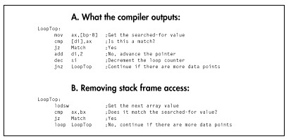
to something like Figure 8.1A. You might look at that and tweak it to the code shown in Figure 8.1B.
Congratulations! You’ve successfully eliminated all stack frame
access, you’ve used LOOP (although DEC SI/JNZ
is actually faster on 386 and later machines, as I explained in the last
chapter), and you’ve used a string instruction. Unfortunately, the new
code isn’t going to run very much faster. Maybe 25 percent faster, maybe
a little more. Big deal. You’ve eliminated the trappings of the
compiler—the stack frame and the restricted register usage—but you’re
still thinking like the compiler. Try this:
repnz scasw
jz MatchIt’s a simple example—but, I hope, a convincing one. Stretch your brain when you optimize.
Taking It to the Limit
The ultimate in assembly language optimization comes when you change
the rules; that is, when you reorganize the entire program to allow the
use of better assembly language code in the small section of code that
most affects overall performance. For example, consider that the data
searched in the last example is stored in an array of structures, with
each structure in the array containing other information as well. In
this situation, REP SCASW couldn’t be used because the data
searched through wouldn’t be contiguous.
However, if the need for performance in searching the array is urgent
enough, there’s no reason why you can’t reorganize the data. This might
mean removing the array elements from the structures and storing them in
their own array so that REP SCASW could be
used.
More on this shortly.
To recap, here are some things to look for when striving to convert C code into optimized assembly language:
- Move the entire performance-critical section into a single assembly language function.
- Don’t use calls or stack frame accesses inside the critical code, if possible, and avoid unnecessary memory accesses of any kind.
- Change segments as infrequently as possible.
- Optimize in terms of what assembly does well, not in terms of fine-tuning compiled C code.
- Change the rules to the benefit of assembly, if necessary; for example, reorganize data structto allow efficient assembly language processing.
That said, let me show some of these precepts in action.
A C-to-Assembly Case Study
Listing 8.1 is the sample C application I’m going to use to examine
optimization in action. Listing 8.1 isn’t really complete—it doesn’t
handle the “no-matches” case well, and it assumes that the sum of all
matches will fit into an int-but it will do just fine as an
optimization example.
LISTING 8.1 L8-1.C
/* Program to search an array spanning a linked list of variable-
sized blocks, for all entries with a specified ID number,
and return the average of the values of all such entries. Each of
the variable-sized blocks may contain any number of data entries,
stored as an array of structures within the block. */
#include <stdio.h>
#ifdef __TURBOC__
#include <alloc.h>
#else
#include <malloc.h>
#endif
void main(void);
void exit(int);
unsigned int FindIDAverage(unsigned int, struct BlockHeader *);
/* Structure that starts each variable-sized block */
struct BlockHeader {
struct BlockHeader *NextBlock; /* Pointer to next block, or NULL
if this is the last block in the
linked list */
unsigned int BlockCount; /* The number of DataElement entries
in this variable-sized block */
};
/* Structure that contains one element of the array we'll search */
struct DataElement {
unsigned int ID; /* ID # for array entry */
unsigned int Value; /* Value of array entry */
};
void main(void) {
int i,j;
unsigned int IDToFind;
struct BlockHeader *BaseArrayBlockPointer,*WorkingBlockPointer;
struct DataElement *WorkingDataPointer;
struct BlockHeader **LastBlockPointer;
printf("ID # for which to find average: ");
scanf("%d",&IDToFind);
/* Build an array across 5 blocks, for testing */
/* Anchor the linked list to BaseArrayBlockPointer */
LastBlockPointer = &BaseArrayBlockPointer;
/* Create 5 blocks of varying sizes */
for (i = 1; i < 6; i++) {
/* Try to get memory for the next block */
if ((WorkingBlockPointer =
(struct BlockHeader *) malloc(sizeof(struct BlockHeader) +
sizeof(struct DataElement) * i * 10)) == NULL) {
exit(1);
}
/* Set the # of data elements in this block */
WorkingBlockPointer->BlockCount = i * 10;
/* Link the new block into the chain */
*LastBlockPointer = WorkingBlockPointer;
/* Point to the first data field */
WorkingDataPointer =
(struct DataElement *) ((char *)WorkingBlockPointer +
sizeof(struct BlockHeader));
/* Fill the data fields with ID numbers and values */
for (j = 0; j < (i * 10); j++, WorkingDataPointer++) {
WorkingDataPointer->ID = j;
WorkingDataPointer->Value = i * 1000 + j;
}
/* Remember where to set link from this block to the next */
LastBlockPointer = &WorkingBlockPointer->NextBlock;
}
/* Set the last block's "next block" pointer to NULL to indicate
that there are no more blocks */
WorkingBlockPointer->NextBlock = NULL;
printf("Average of all elements with ID %d: %u\n",
IDToFind, FindIDAverage(IDToFind, BaseArrayBlockPointer));
exit(0);
}
/* Searches through the array of DataElement entries spanning the
linked list of variable-sized blocks, starting with the block
pointed to by BlockPointer, for all entries with IDs matching
SearchedForID, and returns the average value of those entries. If
no matches are found, zero is returned */
unsigned int FindIDAverage(unsigned int SearchedForID,
struct BlockHeader *BlockPointer)
{
struct DataElement *DataPointer;
unsigned int IDMatchSum;
unsigned int IDMatchCount;
unsigned int WorkingBlockCount;
IDMatchCount = IDMatchSum = 0;
/* Search through all the linked blocks until the last block
(marked with a NULL pointer to the next block) has been
searched */
do {
/* Point to the first DataElement entry within this block */
DataPointer =
(struct DataElement *) ((char *)BlockPointer +
sizeof(struct BlockHeader));
/* Search all the DataElement entries within this block
and accumulate data from all that match the desired ID */
for (WorkingBlockCount=0;
WorkingBlockCount<BlockPointer->BlockCount;
WorkingBlockCount++, DataPointer++) {
/* If the ID matches, add in the value and increment the
match counter */
if (DataPointer->ID == SearchedForID) {
IDMatchCount++;
IDMatchSum += DataPointer->Value;
}
}
/* Point to the next block, and continue as long as that pointer
isn't NULL */
} while ((BlockPointer = BlockPointer->NextBlock) != NULL);
/* Calculate the average of all matches */
if (IDMatchCount == 0)
return(0); /* Avoid division by 0 */
else
return(IDMatchSum / IDMatchCount);
}The main body of Listing 8.1 constructs a linked list of memory
blocks of various sizes and stores an array of structures across those
blocks, as shown in Figure 8.2. The function FindIDAverage
in Listing 8.1 searches through that array for all matches to a
specified ID number and returns the average value of all such matches.
FindIDAverage contains two nested loops, the outer one
repeating once for each linked block and the inner one repeating once
for each array element in each block. The inner loop—the critical one—is
compact, containing only four statements, and should lend itself rather
well to compiler optimization.
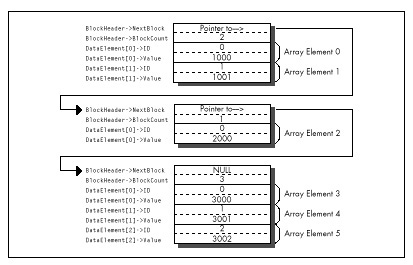
As it happens, Microsoft C/C++ does optimize the inner loop of
FindIDAverage nicely. Listing 8.2 shows the code Microsoft
C/C++ generates for the inner loop, consisting of a mere seven assembly
language instructions inside the loop. The compiler is smart enough to
convert the loop index variable, which counts up but is used for nothing
but counting loops, into a count-down variable so that the
LOOP instruction can be used.
LISTING 8.2 L8-2.COD
; Code generated by Microsoft C for inner loop of FindIDAverage.
;|*** for (WorkingBlockCount=0;
;|*** WorkingBlockCount<BlockPointer->BlockCount;
;|*** WorkingBlockCount++, DataPointer++) {
mov WORD PTR [bp-6],0 ;WorkingBlockCount
mov bx,WORD PTR [bp+6] ;BlockPointer
cmp WORD PTR [bx+2],0
je $FB264
mov cx,WORD PTR [bx+2]
add WORD PTR [bp-6],cx ;WorkingBlockCount
mov di,WORD PTR [bp-2] ;IDMatchSum
mov dx,WORD PTR [bp-4] ;IDMatchCount
$L20004:
;|*** if (DataPointer->ID == SearchedForID) {
mov ax,WORD PTR [si]
cmp WORD PTR [bp+4],ax ;SearchedForID
jne $I265
;|*** IDMatchCount++;
inc dx
;|*** IDMatchSum += DataPointer->Value;
add di,WORD PTR [si+2]
;|*** }
;|*** }
$I265:
add si,4
loop $L20004
mov WORD PTR [bp-2],di ;IDMatchSum
mov WORD PTR [bp-4],dx ;IDMatchCount
$FB264:It’s hard to squeeze much more performance from this code by tweaking
it, as exemplified by Listing 8.3, a fine-tuned assembly version of
FindIDAverage that was produced by looking at the assembly
output of MS C/C++ and tightening it. Listing 8.3 eliminates all stack
frame access in the inner loop, but that’s about all the tightening
there is to do. The result, as shown in Table 8.1, is that Listing 8.3
runs a modest 11 percent faster than Listing 8.1 on a 386. The results
could vary considerably, depending on the nature of the data set
searched through (average block size and frequency of matches). But,
then, understanding the typical and worst case conditions is part of
optimization, isn’t it?
LISTING 8.3 L8-3.ASM
; Typically optimized assembly language version of FindIDAverage.
SearchedForID equ 4 ;Passed parameter offsets in the
BlockPointer equ 6 ; stack frame (skip over pushed BP
; and the return address)
NextBlock equ 0 ;Field offsets in struct BlockHeader
BlockCount equ 2
BLOCK_HEADER_SIZE equ 4 ;Number of bytes in struct BlockHeader
ID equ 0 ;struct DataElement field offsets
Value equ 2
DATA_ELEMENT_SIZE equ 4 ;Number of bytes in struct DataElement
.model small
.code
public _FindIDAverage| On 20 MHz 386 | On 10 MHz 286 | |
|---|---|---|
| Listing 8.1 (MSC with maximum optimization) | 294 microseconds | 768 microseconds |
| Listing 8.3 (Assembly) | 265 | 644 |
| Listing 8.4 (Optimized assembly) | 212 | 486 |
| Listing 8.6 (Optimized assembly with reorganized data) | 100 | 207 |
_FindIDAverage proc near
push bp ;Save caller's stack frame
mov bp,sp ;Point to our stack frame
push di ;Preserve C register variables
push si
sub dx,dx ;IDMatchSum = 0
mov bx,dx ;IDMatchCount = 0
mov si,[bp+BlockPointer] ;Pointer to first block
mov ax,[bp+SearchedForID] ;ID we're looking for
; Search through all the linked blocks until the last block
; (marked with a NULL pointer to the next block) has been searched.
BlockLoop:
; Point to the first DataElement entry within this block.
lea di,[si+BLOCK_HEADER_SIZE]
; Search through all the DataElement entries within this block
; and accumulate data from all that match the desired ID.
mov cx,[si+BlockCount]
jcxz DoNextBlock ;No data in this block
IntraBlockLoop:
cmp [di+ID],ax ;Do we have an ID match?
jnz NoMatch ;No match
inc bx ;We have a match; IDMatchCount++;
add dx,[di+Value] ;IDMatchSum += DataPointer->Value;
NoMatch:
add di,DATA_ELEMENT_SIZE ;point to the next element
loop IntraBlockLoop
; Point to the next block and continue if that pointer isn't NULL.
DoNextBlock:
mov si,[si+NextBlock] ;Get pointer to the next block
and si,si ;Is it a NULL pointer?
jnz BlockLoop ;No, continue
; Calculate the average of all matches.
sub ax,ax ;Assume we found no matches
and bx,bx
jz Done ;We didn't find any matches, return 0
xchg ax,dx ;Prepare for division
div bx ;Return IDMatchSum / IDMatchCount
Done: pop si ;Restore C register variables
pop di
pop bp ;Restore caller's stack frame
ret
_FindIDAverage ENDP
endListing 8.4 tosses some sophisticated optimization techniques into
the mix. The loop is unrolled eight times, eliminating a good deal of
branching, and SCASW is used instead of
CMP [DI],AX. (Note, however, that SCASW is in
fact slower than CMP [DI],AX on the 386 and 486, and is
sometimes faster on the 286 and 8088 only because it’s shorter and
therefore may prefetch faster.) This advanced tweaking produces a 39
percent improvement over the original C code—substantial, but not a
tremendous return for the optimization effort invested.
LISTING 8.4 L8-4.ASM
; Heavily optimized assembly language version of FindIDAverage.
; Features an unrolled loop and more efficient pointer use.
SearchedForID equ 4 ;Passed parameter offsets in the
BlockPointer equ 6 ; stack frame (skip over pushed BP
; and the return address)
NextBlock equ 0 ;Field offsets in struct BlockHeader
BlockCount equ 2
BLOCK_HEADER_SIZE equ 4 ;Number of bytes in struct BlockHeader
ID equ 0 ;struct DataElement field offsets
Value equ 2
DATA_ELEMENT_SIZE equ 4 ;Number of bytes in struct DataElement
.model small
.code
public _FindIDAverage
_FindIDAverage proc near
push bp ;Save caller's stack frame
mov bp,sp ;Point to our stack frame
push di ;Preserve C register variables
push si
mov di,ds ;Prepare for SCASW
mov es,di
cld
sub dx,dx ;IDMatchSum = 0
mov bx,dx ;IDMatchCount = 0
mov si,[bp+BlockPointer] ;Pointer to first block
mov ax,[bp+SearchedForID] ;ID we're looking for
; Search through all of the linked blocks until the last block
; (marked with a NULL pointer to the next block) has been searched.
BlockLoop:
; Point to the first DataElement entry within this block.
lea di,[si+BLOCK_HEADER_SIZE]
; Search through all the DataElement entries within this block
; and accumulate data from all that match the desired ID.
mov cx,[si+BlockCount] ;Number of elements in this block
jcxz DoNextBlock ;Skip this block if it's empty
mov bp,cx ;***stack frame no longer available***
add cx,7
shr cx,1 ;Number of repetitions of the unrolled
shr cx,1 ; loop = (BlockCount + 7) / 8
shr cx,1
and bp,7 ;Generate the entry point for the
shl bp,1 ; first, possibly partial pass through
jmp cs:[LoopEntryTable+bp] ; the unrolled loop and
; vector to that entry point
align 2
LoopEntryTable label word
dw LoopEntry8,LoopEntry1,LoopEntry2,LoopEntry3
dw LoopEntry4,LoopEntry5,LoopEntry6,LoopEntry7
M_IBL macro P1
local NoMatch
LoopEntry&P1&:
scasw ;Do we have an ID match?
jnz NoMatch ;No match
;We have a match
inc bx ;IDMatchCount++;
add dx,[di] ;IDMatchSum += DataPointer->Value;
NoMatch:
add di,DATA_ELEMENT_SIZE-2 ;point to the next element
; (SCASW advanced 2 bytes already)
endm
align 2
IntraBlockLoop:
M_IBL 8
M_IBL 7
M_IBL 6
M_IBL 5
M_IBL 4
M_IBL 3
M_IBL 2
M_IBL 1
loop IntraBlockLoop
; Point to the next block and continue if that pointer isn't NULL.
DoNextBlock:
mov si,[si+NextBlock] ;Get pointer to the next block
and si,si ;Is it a NULL pointer?
jnz BlockLoop ;No, continue
; Calculate the average of all matches.
sub ax,ax ;Assume we found no matches
and bx,bx
jz Done ;We didn't find any matches, return 0
xchg ax,dx ;Prepare for division
div bx ;Return IDMatchSum / IDMatchCount
Done: pop si ;Restore C register variables
pop di
pop bp ;Restore caller's stack frame
ret
_FindIDAverage ENDP
endListings 8.5 and 8.6 together go the final step and change the rules in favor of assembly language. Listing 8.5 creates the same list of linked blocks as Listing 8.1. However, instead of storing an array of structures within each block, it stores two arrays in each block, one consisting of ID numbers and the other consisting of the corresponding values, as shown in Figure 8.3. No information is lost; the data is merely rearranged.
LISTING 8.5 L8-5.C
/* Program to search an array spanning a linked list of variable-
sized blocks, for all entries with a specified ID number,
and return the average of the values of all such entries. Each of
the variable-sized blocks may contain any number of data entries,
stored in the form of two separate arrays, one for ID numbers and
one for values. */
#include <stdio.h>
#ifdef __TURBOC__
#include <alloc.h>
#else
#include <malloc.h>
#endif
void main(void);
void exit(int);
extern unsigned int FindIDAverage2(unsigned int,
struct BlockHeader *);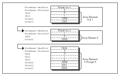
/* Structure that starts each variable-sized block */
struct BlockHeader {
struct BlockHeader *NextBlock; /* Pointer to next block, or NULL
if this is the last block in the
linked list */
unsigned int BlockCount; /* The number of DataElement entries
in this variable-sized block */
};
void main(void) {
int i,j;
unsigned int IDToFind;
struct BlockHeader *BaseArrayBlockPointer,*WorkingBlockPointer;
int *WorkingDataPointer;
struct BlockHeader **LastBlockPointer;
printf("ID # for which to find average: ");
scanf("%d",&IDToFind);
/* Build an array across 5 blocks, for testing */
/* Anchor the linked list to BaseArrayBlockPointer */
LastBlockPointer = &BaseArrayBlockPointer;
/* Create 5 blocks of varying sizes */
for (i = 1; i < 6; i++) {
/* Try to get memory for the next block */
if ((WorkingBlockPointer =
(struct BlockHeader *) malloc(sizeof(struct BlockHeader) +
sizeof(int) * 2 * i * 10)) == NULL) {
exit(1);
}
/* Set the number of data elements in this block */
WorkingBlockPointer->BlockCount = i * 10;
/* Link the new block into the chain */
*LastBlockPointer = WorkingBlockPointer;
/* Point to the first data field */
WorkingDataPointer = (int *) ((char *)WorkingBlockPointer +
sizeof(struct BlockHeader));
/* Fill the data fields with ID numbers and values */
for (j = 0; j < (i * 10); j++, WorkingDataPointer++) {
*WorkingDataPointer = j;
*(WorkingDataPointer + i * 10) = i * 1000 + j;
}
/* Remember where to set link from this block to the next */
LastBlockPointer = &WorkingBlockPointer->NextBlock;
}
/* Set the last block's "next block" pointer to NULL to indicate
that there are no more blocks */
WorkingBlockPointer->NextBlock = NULL;
printf("Average of all elements with ID %d: %u\n",
IDToFind, FindIDAverage2(IDToFind, BaseArrayBlockPointer));
exit(0);
}LISTING 8.6 L8-6.ASM
; Alternative optimized assembly language version of FindIDAverage
; requires data organized as two arrays within each block rather
; than as an array of two-value element structures. This allows the
; use of REP SCASW for ID searching.
SearchedForIDequ4 ;Passed parameter offsets in the
BlockPointerequ6 ; stack frame (skip over pushed BP
; and the return address)
NextBlockequ0 ;Field offsets in struct BlockHeader
BlockCountequ2
BLOCK_HEADER_SIZEequ4 ;Number of bytes in struct BlockHeader
.model small
.code
public _FindIDAverage2
_FindIDAverage2 proc near
push bp ;Save caller's stack frame
mov bp,sp ;Point to our stack frame
push di ;Preserve C register variables
push si
mov di,ds ;Prepare for SCASW
mov es,di
cld
mov si,[bp+BlockPointer] ;Pointer to first block
mov ax,[bp+SearchedForID] ;ID we're looking for
sub dx,dx ;IDMatchSum = 0
mov bp,dx ;IDMatchCount = 0
;***stack frame no longer available***
; Search through all the linked blocks until the last block
; (marked with a NULL pointer to the next block) has been searched.
BlockLoop:
; Search through all the DataElement entries within this block
; and accumulate data from all that match the desired ID.
mov cx,[si+BlockCount]
jcxz DoNextBlock;Skip this block if there's no data
; to search through
mov bx,cx ;We'll use BX to point to the
shl bx,1 ; corresponding value entry in the
; case of an ID match (BX is the
; length in bytes of the ID array)
; Point to the first DataElement entry within this block.
lea di,[si+BLOCK_HEADER_SIZE]
IntraBlockLoop:
repnz scasw ;Search for the ID
jnz DoNextBlock ;No match, the block is done
inc bp ;We have a match; IDMatchCount++;
add dx,[di+bx-2];IDMatchSum += DataPointer->Value;
; (SCASW has advanced DI 2 bytes)
and cx,cx ;Is there more data to search through?
jnz IntraBlockLoop ;yes
; Point to the next block and continue if that pointer isn't NULL.
DoNextBlock:
mov si,[si+NextBlock] ;Get pointer to the next block
and si,si ;Is it a NULL pointer?
jnz BlockLoop ;No, continue
; Calculate the average of all matches.
sub ax,ax ;Assume we found no matches
and bp,bp
jz Done ;We didn't find any matches, return 0
xchg ax,dx ;Prepare for division
div bp ;Return IDMatchSum / IDMatchCount
Done: pop si ;Restore C register variables
pop di
pop bp ;Restore caller's stack frame
ret
_FindIDAverage2 ENDP
endThe whole point of this rearrangement is to allow us to use
REP SCASW to search through each block, and that’s exactly
what FindIDAverage2 in Listing 8.6 does. The result:
Listing 8.6 calculates the average about three times as fast as
the original C implementation and more than twice as fast as Listing
8.4, heavily optimized as the latter code is.
I trust you get the picture. The sort of instruction-by-instruction optimization that so many of us love to do as a kind of puzzle is fun, but compilers can do it nearly as well as you can, and in the future will surely do it better. What a compiler can’t do is tie together the needs of the program specification on the high end and the processor on the low end, resulting in critical code that runs just about as fast as the hardware permits. The only software that can do that is located north of your sternum and slightly aft of your nose. Dust it off and put it to work—and your code will never again be confused with anything by Hamilton, Joe, Frank, eynolds or Bo Donaldson and the Heywoods.
Chapter 9 – Hints My Readers Gave Me
Optimization Odds and Ends from the Field
Back in high school, I took a pre-calculus class from Mr. Bourgeis, whose most notable characteristics were incessant pacing and truly enormous feet. My friend Barry, who sat in the back row, right behind me, claimed that it was because of his large feet that Mr. Bourgeis was so restless. Those feet were so heavy, Barry hypothesized, that if Mr. Bourgeis remained in any one place for too long, the floor would give way under the strain, plunging the unfortunate teacher deep into the mantle of the Earth and possibly all the way through to China. Many amusing cartoons were drawn to this effect.
Unfortunately, Barry was too busy drawing cartoons, or, alternatively, sleeping, to actually learn any math. In the long run, that didn’t turn out to be a handicap for Barry, who went on to become vice-president of sales for a ham-packing company, where presumably he was rarely called upon to derive the quadratic equation. Barry’s lack of scholarship caused some problems back then, though. On one memorable occasion, Barry was half-asleep, with his eyes open but unfocused and his chin balanced on his hand in the classic “if I fall asleep my head will fall off my hand and I’ll wake up” posture, when Mr. Bourgeis popped a killer problem:
“Barry, solve this for X, please.” On the blackboard lay the equation:
X - 1 = 0“Minus 1,” Barry said promptly.
Mr. Bourgeis shook his head mournfully. “Try again.” Barry thought hard. He knew the fundamental rule that the answer to most mathematical questions is either 0, 1, infinity, -1, or minus infinity (do not apply this rule to balancing your checkbook, however); unfortunately, that gave him only a 25 percent chance of guessing right.
“One,” I whispered surreptitiously.
“Zero,” Barry announced. Mr. Bourgeis shook his head even more sadly.
“One,” I whispered louder. Barry looked still more thoughtful—a bad sign—so I whispered “one” again, even louder. Barry looked so thoughtful that his eyes nearly rolled up into his head, and I realized that he was just doing his best to convince Mr. Bourgeis that Barry had solved this one by himself.
As Barry neared the climax of his stirring performance and opened his mouth to speak, Mr. Bourgeis looked at him with great concern. “Barry, can you hear me all right?”
“Yes, sir,” Barry replied. “Why?”
“Well, I could hear the answer all the way up here. Surely you could hear it just one row away?”
The class went wild. They might as well have sent us home early for all we accomplished the rest of the day.
I like to think I know more about performance programming than Barry knew about math. Nonetheless, I always welcome good ideas and comments, and many readers have sent me a slew of those over the years. So in this chapter, I think I’ll return the favor by devoting a chapter to reader feedback.
Another Look at LEA
Several people have pointed out that while LEA is great
for performing certain additions (see Chapter 6), it isn’t a perfect
replacement for ADD. What’s the difference?
LEA, an addressing instruction by trade, doesn’t affect the
flags, while the arithmetic ADD instruction most certainly
does. This is no problem when performing additions that involve only
quantities that fit in one machine word (32 bits in 386 protected mode,
16 bits otherwise), but it renders LEA useless for
multiword operations, which use the Carry flag to tie together partial
results. For example, these instructions
ADD EAX,EBX
ADC EDX,ECXcould not be replaced
LEA EAX,[EAX+EBX]
ADC EDX,ECXbecause LEA doesn’t affect the Carry flag.
The no-carry characteristic of LEA becomes a distinct
advantage when performing pointer arithmetic, however. For instance, the
following code uses LEA to advance the pointers while
adding one 128-bit memory variable to another such variable:
MOV ECX,4 ;# of 32-bit words to add
CLC
;no carry into the initial ADC
ADDLOOP:
MOV EAX,[ESI] ;get the next element of one array
ADC [EDI],EAX ;add it to the other array, with carry
LEA ESI,[ESI+4] ;advance one array's pointer
LEA EDI,[EDI+4] ;advance the other array's pointer
LOOP ADDLOOP(Yes, I could use LODSD instead of MOV/LEA;
I’m just illustrating a point here. Besides, LODS is only 1
cycle faster than MOV/LEA on the 386, and is actually more
than twice as slow on the 486.) If we used ADD rather than
LEA to advance the pointers, the carry from one
ADC to the next would have to be preserved with either
PUSHF/POPF or LAHF/SAHF. (Alternatively, we
could use multiple INCs, since INC doesn’t
affect the Carry flag.)
In short, LEA is indeed different from ADD.
Sometimes it’s better. Sometimes not; that’s the nature of the various
instruction substitutions and optimizations that will occur to you over
time. There’s no such thing as “best” instructions on the x86; it all
depends on what you’re trying to do.
But there sure are a lot of interesting options, aren’t there?
The Kennedy Portfolio
Reader John Kennedy regularly passes along intriguing assembly programming tricks, many of which I’ve never seen mentioned anywhere else. John likes to optimize for size, whereas I lean more toward speed, but many of his optimizations are good for both purposes. Here are a few of my favorites:
John’s code for setting AX to its absolute value is:
CWD
XOR AX,DX
SUB AX,DXThis does nothing when bit 15 of AX is 0 (that is, if AX is positive). When AX is negative, the code “nots” it and adds 1, which is exactly how you perform a two’s complement negate. For the case where AX is not negative, this trick usually beats the stuffing out of the standard absolute value code:
AND AX,AX ;negative?
JNS IsPositive ;no
NEG AX ;yes,negate it
IsPositive:However, John’s code is slower on a 486; as you’re no doubt coming to realize (and as I’ll explain in Chapters 12 and 13), the 486 is an optimization world unto itself.
Here’s how John copies a block of bytes from DS:SI to ES:DI, moving as much data as possible a word at a time:
SHR CX,1 ;word count
REP MOVSW ;copy as many words as possible
ADC CX,CX ;CX=1 if copy length was odd,
;0 else
REP MOVSB ;copy any odd byte(ADC CX,CX can be replaced with RCL CX,1;
which is faster depends on the processor type.) It might be hard to
believe that the above is faster than this:
SHR CX,1 ;word count
REP MOVSW ;copy as many words as
;possible
JNC CopyDone ;done if even copy length
MOVSB ;copy the odd byte
CopyDone:However, it generally is. Sure, if the length is odd, John’s approach
incurs a penalty approximately equal to the REP startup
time for MOVSB. However, if the length is even, John’s
approach doesn’t branch, saving cycles and not emptying the prefetch
queue. If copy lengths are evenly distributed between even and odd,
John’s approach is faster in most x86 systems. (Not on the 486,
though.)
John also points out that on the 386, multiple LEAs can
be combined to perform multiplications that can’t be handled by a single
LEA, much as multiple shifts and adds can be used for
multiplication, only faster. LEA can be used to multiply in
a single instruction on the 386, but only by the values 2, 3, 4, 5, 8,
and 9; several LEAs strung together can handle a much wider
range of values. For example, video programmers are undoubtedly familiar
with the following code to multiply AX times 80 (the width in bytes of
the bitmap in most PC display modes):
SHL AX,1 ;*2
SHL AX,1 ;*4
SHL AX,1 ;*8
SHL AX,1 ;*16
MOV BX,AX
SHL AX,1 ;*32
SHL AX,1 ;*64
ADD AX,BX ;*80Using LEA on the 386, the above could be reduced to
LEA EAX,[EAX*2] ;*2
LEA EAX,[EAX*8] ;*16
LEA EAX,[EAX+EAX*4] ;*80which still isn’t as fast as using a lookup table like
MOV EAX,MultiplesOf80Table[EAX*4]but is close and takes a great deal less space.
Of course, on the 386, the shift and add version could also be reduced to this considerably more efficient code:
SHL AX,4 ;*16
MOV BX,AX
SHL AX,2 ;*64
ADD AX,BX ;*80Speeding Up Multiplication
That brings us to multiplication, one of the slowest of x86
operations and one that allows for considerable optimization. One way to
speed up multiplication is to use shift and add, LEA, or a
lookup table to hard-code a multiplication operation for a fixed
multiplier, as shown above. Another is to take advantage of the
early-out feature of the 386 (and the 486, but in the interests of
brevity I’ll just say “386” from now on) by arranging your operands so
that the multiplier (always the rightmost operand following
MUL or IMUL) is no larger than the other
operand.
(There’s a minimum execution time on this trick; below 3 significant multiplier bits, no additional cycles are saved.) For example, multiplication of 32,767 times 1 is 12 cycles faster than multiplication of 1 times 32,727.
Choosing the right operand as the multiplier can work wonders. According to published specs, the 386 takes 38 cycles to multiply by a multiplier with 32 significant bits but only 9 cycles to multiply by a multiplier of 2, a performance improvement of more than four times! (My tests regularly indicate that multiplication takes 3 to 4 cycles longer than the specs indicate, but the cycle-per-bit advantage of smaller multipliers holds true nonetheless.)
This highlights another interesting point: MUL and
IMUL on the 386 are so fast that alternative multiplication
approaches, while generally still faster, are worthwhile only in truly
time-critical code.
MULandIMULinstructions can approach and in some cases even outperform the “optimized” alternatives.
All in all, MUL and IMUL are reasonable
performers on the 386, no longer to be avoided in most cases—and you can
help that along by arranging your code to make the smaller operand the
multiplier whenever you know which operand is smaller.
That doesn’t mean that your code should test and swap operands to make sure the smaller one is the multiplier; that rarely pays off. I’m speaking more of the case where you’re scaling an array up by a value that’s always in the range of, say, 2 to 10; because the scale value will always be small and the array elements may have any value, the scale value is the logical choice for the multiplier.
Optimizing Optimized Searching
Rob Williams writes with a wonderful optimization to the
REPNZ SCASB-based optimized searching routine I discussed
in Chapter 5. As a quick refresher, I described searching a buffer for a
text string as follows: Scan for the first byte of the text string with
REPNZ SCASB, then use REPZ CMPS to check for a
full match whenever REPNZ SCASB finds a match for the first
character, as shown in Figure 9.1. The principle is that most buffer
characters won’t match the first character of any given string, so
REPNZ SCASB, by far the fastest way to search on the PC,
can be used to eliminate most potential matches; each remaining
potential match can then be checked in its entirety with
REPZ CMPS.
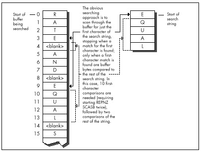
Rob’s revelation, which he credits without explanation to Edgar Allen
Poe (search nevermore?), was that by far the slowest part of the whole
deal is handling REPNZ SCASB matches, which require
checking the remainder of the string with REPZ CMPS and
restarting REPNZ SCASB if no match is found.
REPNZ SCASBmatches can easily be reduced simply by scanning for the character in the searched-for string that appears least often in the buffer being searched.
Imagine, if you will, that you’re searching for the string “EQUAL.”
By my approach, you’d use REPNZ SCASB to scan for each
occurrence of “E,” which crops up quite often in normal text. Rob points
out that it would make more sense to scan for “Q,” then back up one
character and check the whole string when a “Q” is found, as shown in
Figure 9.2. “Q” is likely to occur much less often, resulting in many
fewer whole-string checks and much faster processing.
Listing 9.1 implements the scan-on-first-character approach. Listing
9.2 scans for whatever character the caller specifies. Listing 9.3 is a
test program used to compare the two approaches. How much difference
does Rob’s revelation make? Plenty. Even when the entire C function call
to FindString is timed—strlen calls, parameter
pushing, calling, setup, and all—the version of FindString
in Listing 9.2, which is directed by Listing 9.3 to scan for the
infrequently-occurring “Q,” is about 40 percent faster on a 20 MHz
cached 386 for the test search of Listing 9.3 than is the version of
FindString in Listing 9.1, which always scans for the first
character, in this case “E.” However, when only the search loops (the
code that actually does the searching) in the two versions of
FindString are compared, Listing 9.2 is more than
twice as fast as Listing 9.1—a remarkable improvement over code
that already uses REPNZ SCASB and
REPZ CMPS.
What I like so much about Rob’s approach is that it demonstrates that
optimization involves much more than instruction selection and cycle
counting. Listings 9.1 and 9.2 use pretty much the same instructions,
and even use the same approach of scanning with REPNZ SCASB
and using REPZ CMPS to check scanning matches.
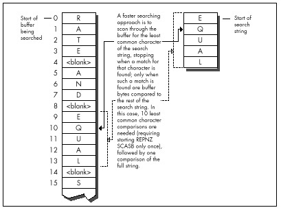
LISTING 9.1 L9-1.ASM
; Searches a text buffer for a text string. Uses REPNZ SCASB to sca"n
; the buffer for locations that match the first character of the
; searched-for string, then uses REPZ CMPS to check fully only those
; locations that REPNZ SCASB has identified as potential matches.
;
; Adapted from Zen of Assembly Language, by Michael Abrash
;
; C small model-callable as:
; unsigned char * FindString(unsigned char * Buffer,
; unsigned int BufferLength, unsigned char * SearchString,
; unsigned int SearchStringLength);
;
; Returns a pointer to the first match for SearchString in Buffer,or
; a NULL pointer if no match is found. Buffer should not start at
; offset 0 in the data segment to avoid confusing a match at 0 with
; no match found.
Parmsstruc
dw 2 dup(?) ;pushed BP/return address
Buffer dw ? ;pointer to buffer to search
BufferLength dw ? ;length of buffer to search
SearchString dw ? ;pointer to string for which to search
SearchStringLength dw ? ;length of string for which to search
Parmsends
.model small
.code
public _FindString
_FindString proc near
push bp ;preserve caller's stack frame
mov bp,sp ;point to our stack frame
push si ;preserve caller's register variables
push di
cld ;make string instructions increment pointers
mov si,[bp+SearchString] ;pointer to string to search for
mov bx,[bp+SearchStringLength] ;length of string
and bx,bx
jz FindStringNotFound ;no match if string is 0 length
movd x,[bp+BufferLength] ;length of buffer
sub dx,bx ;difference between buffer and string lengths
jc FindStringNotFound ;no match if search string is
; longer than buffer
inc dx ;difference between buffer and search string
; lengths, plus 1 (# of possible string start
; locations to check in the buffer)
mov di,ds
mov es,di
mov di,[bp+Buffer] ;point ES:DI to buffer to search thru
lodsb ;put the first byte of the search string in AL
mov bp,si ;set aside pointer to the second search byte
dec bx ;don't need to compare the first byte of the
; string with CMPS; we'll do it with SCAS
FindStringLoop:
mov cx,dx ;put remaining buffer search length in CX
repnz scasb ;scan for the first byte of the string
jnz FindStringNotFound ;not found, so there's no match
;found, so we have a potential match-check the
; rest of this candidate location
push di ;remember the address of the next byte to scan
mov dx,cx ;set aside the remaining length to search in
; the buffer
mov si,bp ;point to the rest of the search string
mov cx,bx ;string length (minus first byte)
shr cx,1 ;convert to word for faster search
jnc FindStringWord ;do word search if no odd byte
cmpsb ;compare the odd byte
jnz FindStringNoMatch ;odd byte doesn't match, so we
; haven't found the search string here
FindStringWord:
jcxz FindStringFound ;test whether we've already checked
; the whole string; if so, this is a match
; bytes long; if so, we've found a match
repz cmpsw ;check the rest of the string a word at a time
jz FindStringFound ;it's a match
FindStringNoMatch:
pop di ;get back pointer to the next byte to scan
and dx,dx ;is there anything left to check?
jnz FindStringLoop ;yes-check next byte
FindStringNotFound:
sub ax,ax ;return a NULL pointer indicating that the
jmp FindStringDone ; string was not found
FindStringFound:
pop ax ;point to the buffer location at which the
dec ax ; string was found (earlier we pushed the
; address of the byte after the start of the
; potential match)
FindStringDone:
pop di ;restore caller's register variables
pop si
pop bp ;restore caller's stack frame
ret
_FindString endp
endLISTING 9.2 L9-2.ASM
; Searches a text buffer for a text string. Uses REPNZ SCASB to scan
; the buffer for locations that match a specified character of the
; searched-for string, then uses REPZ CMPS to check fully only those
; locations that REPNZ SCASB has identified as potential matches.
;
; C small model-callable as:
; unsigned char * FindString(unsigned char * Buffer,
; unsigned int BufferLength, unsigned char * SearchString,
; unsigned int SearchStringLength,
; unsigned int ScanCharOffset);
;
; Returns a pointer to the first match for SearchString in Buffer,or
; a NULL pointer if no match is found. Buffer should not start at
; offset 0 in the data segment to avoid confusing a match at 0 with
; no match found.
Parms struc
dw 2 dup(?) ;pushed BP/return address
Buffer dw ? ;pointer to buffer to search
BufferLength dw ? ;length of buffer to search
SearchString dw ? ;pointer to string for which to search
SearchStringLength dw ? ;length of string for which to search
ScanCharOffset dw ? ;offset in string of character for
; which to scan
Parmsends
.model small
.code
public _FindString
_FindString proc near
push bp ;preserve caller's stack frame
mov bp,sp ;point to our stack frame
push si ;preserve caller's register variables
push di
cld ;make string instructions increment pointers
mov si,[bp+SearchString] ;pointer to string to search for
mov cx,[bp+SearchStringLength] ;length of string
jcxz FindStringNotFound ;no match if string is 0 length
mov dx,[bp+BufferLength] ;length of buffer
sub dx,cx ;difference between buffer and search
; lengths
jc FindStringNotFound ;no match if search string is
; longer than buffer
inc dx ; difference between buffer and search string
; lengths, plus 1 (# of possible string start
; locations to check in the buffer)
mov di,ds
mov es,di
mov di,[bp+Buffer] ;point ES:DI to buffer to search thru
mov bx,[bp+ScanCharOffset] ;offset in string of character
; on which to scan
add di,bx ;point ES:DI to first buffer byte to scan
mov al,[si+bx] ;put the scan character in AL
inc bx ;set BX to the offset back to the start of the
; potential full match after a scan match,
; accounting for the 1-byte overrun of
; REPNZ SCASB
FindStringLoop:
mov cx,dx ;put remaining buffer search length in CX
repnz scasb ;scan for the scan byte
jnz FindStringNotFound ;not found, so there's no match
;found, so we have a potential match-check the
; rest of this candidate location
push di ;remember the address of the next byte to scan
mov dx,cx ;set aside the remaining length to search in
; the buffer
sub di,bx ;point back to the potential start of the
; match in the buffer
mov si,[bp+SearchString] ;point to the start of the string
mov cx,[bp+SearchStringLength] ;string length
shr cx,1 ;convert to word for faster search
jnc FindStringWord ;do word search if no odd byte
cmpsb ;compare the odd byte
jnz FindStringNoMatch ;odd byte doesn't match, so we
; haven't found the search string here
FindStringWord:
jcxz FindStringFound ;if the string is only 1 byte long,
; we've found a match
repz cmpsw ;check the rest of the string a word at a time
jz FindStringFound ;it's a match
FindStringNoMatch:
pop di ;get back pointer to the next byte to scan
and dx,dx ;is there anything left to check?
jnz FindStringLoop ;yes-check next byte
FindStringNotFound:
sub ax,ax ;return a NULL pointer indicating that the
jmp FindStringDone ; string was not found
FindStringFound:
pop ax ;point to the buffer location at which the
sub ax,bx ; string was found (earlier we pushed the
; address of the byte after the scan match)
FindStringDone:
pop di ;restore caller's register variables
pop si
pop bp ;restore caller's stack frame
ret
_FindString endp
endLISTING 9.3 L9-3.C
/* Program to exercise buffer-search routines in Listings 9.1 & 9.2 */
#include <stdio.h>
#include <string.h>
#define DISPLAY_LENGTH 40
extern unsigned char * FindString(unsigned char *, unsigned int,
unsigned char *, unsigned int, unsigned int);
void main(void);
static unsigned char TestBuffer[] = "When, in the course of human \
events, it becomes necessary for one people to dissolve the \
political bands which have connected them with another, and to \
assume among the powers of the earth the separate and equal station \
to which the laws of nature and of nature's God entitle them...";
void main() {
static unsigned char TestString[] = "equal";
unsigned char TempBuffer[DISPLAY_LENGTH+1];
unsigned char *MatchPtr;
/* Search for TestString and report the results */
if ((MatchPtr = FindString(TestBuffer,
(unsigned int) strlen(TestBuffer), TestString,
(unsigned int) strlen(TestString), 1)) == NULL) {
/* TestString wasn't found */
printf("\"%s\" not found\n", TestString);
} else {
/* TestString was found. Zero-terminate TempBuffer; strncpy
won't do it if DISPLAY_LENGTH characters are copied */
TempBuffer[DISPLAY_LENGTH] = 0;
printf("\"%s\" found. Next %d characters at match:\n\"%s\"\n",
TestString, DISPLAY_LENGTH,
strncpy(TempBuffer, MatchPtr, DISPLAY_LENGTH));
}
}You’ll notice that in Listing 9.2 I didn’t use a table of character frequencies in English text to determine the character for which to scan, but rather let the caller make that choice. Each buffer of bytes has unique characteristics, and English-letter frequency could well be inappropriate. What if the buffer is filled with French text? Cyrillic? What if it isn’t text that’s being searched? It might be worthwhile for an application to build a dynamic frequency table for each buffer so that the best scan character could be chosen for each search. Or perhaps not, if the search isn’t time-critical or the buffer is small.
The point is that you can improve performance dramatically by understanding the nature of the data with which you work. (This is equally true for high-level language programming, by the way.) Listing 9.2 is very similar to and only slightly more complex than Listing 9.1; the difference lies not in elbow grease or cycle counting but in the organic integrating optimizer technology we all carry around in our heads.
Short Sorts
David Stafford (recently of Borland and Borland Japan) who happens to be one of the best assembly language programmers I’ve ever met, has written a C-callable routine that sorts an array of integers in ascending order. That wouldn’t be particularly noteworthy, except that David’s routine, shown in Listing 9.4, is exactly 25 bytes long. Look at the code; you’ll keep saying to yourself, “But this doesn’t work…oh, yes, I guess it does.” As they say in the Prego spaghetti sauce ads, it’s in there—and what a job of packing. Anyway, David says that a 24-byte sort routine eludes him, and he’d like to know if anyone can come up with one.
LISTING 9.4 L9-4.ASM
;--------------------------------------------------------------------------
; Sorts an array of ints. C callable (small model). 25 bytes.
; void sort( int num, int a[] );
;
; Courtesy of David Stafford.
;--------------------------------------------------------------------------
.model small
.code
public _sort
top: mov dx,[bx] ;swap two adjacent integers
xchg dx,[bx+2]
xchg dx,[bx]
cmp dx,[bx] ;did we put them in the right order?
jl top ;no, swap them back
inc bx ;go to next integer
inc bx
loop top
_sort: pop dx ;get return address (entry point)
pop cx ;get count
pop bx ;get pointer
push bx ;restore pointer
dec cx ;decrement count
push cx ;save count
push dx ;restore return address
jg top ;if cx > 0
ret
endFull 32-Bit Division
One of the most annoying limitations of the x86 is that while the
dividend operand to the DIV instruction can be 32 bits in
size, both the divisor and the result must be 16 bits. That’s
particularly annoying in regards to the result because sometimes you
just don’t know whether the ratio of the dividend to the divisor is
greater than 64K-1 or not—and if you guess wrong, you get that godawful
Divide By Zero interrupt. So, what is one to do when the result might
not fit in 16 bits, or when the dividend is larger than 32 bits? Fall
back to a software division approach? That will work—but oh so
slowly.
There’s another technique that’s much faster than a pure software approach, albeit not so flexible. This technique allows arbitrarily large dividends and results, but the divisor is still limited to16 bits. That’s not perfect, but it does solve a number of problems, in particular eliminating the possibility of a Divide By Zero interrupt from a too-large result.
This technique involves nothing more complicated than breaking up the division into word-sized chunks, starting with the most significant word of the dividend. The most significant word is divided by the divisor (with no chance of overflow because there are only 16 bits in each); then the remainder is prepended to the next 16 bits of dividend, and the process is repeated, as shown in Figure 9.3. This process is equivalent to dividing by hand, except that here we stop to carry the remainder manually only after each word of the dividend; the hardware divide takes care of the rest. Listing 9.5 shows a function to divide an arbitrarily large dividend by a 16-bit divisor, and Listing 9.6 shows a sample division of a large dividend. Note that the same principle can be applied to handling arbitrarily large dividends in 386 native mode code, but in that case the operation can proceed a dword, rather than a word, at a time.
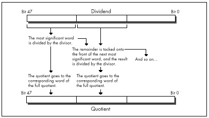
As for handling signed division with arbitrarily large dividends,
that can be done easily enough by remembering the signs of the dividend
and divisor, dividing the absolute value of the dividend by the absolute
value of the divisor, and applying the stored signs to set the proper
signs for the quotient and remainder. There may be more clever ways to
produce the same result, by using IDIV, for example; if you
know of one, drop me a line c/o Coriolis Group Books.
LISTING 9.5 L9-5.ASM
; Divides an arbitrarily long unsigned dividend by a 16-bit unsigned
; divisor. C near-callable as:
; unsigned int Div(unsigned int * Dividend,
; int DividendLength, unsigned int Divisor,
; unsigned int * Quotient);
;
; Returns the remainder of the division.
;
; Tested with TASM 2.
parms struc
dw 2 dup (?) ;pushed BP & return address
Dividend dw ? ;pointer to value to divide, stored in Intel
; order, with lsb at lowest address, msb at
; highest. Must be composed of an integral
; number of words
DividendLength dw ? ;# of bytes in Dividend. Must be a multiple
; of 2
Divisor dw ? ;value by which to divide. Must not be zero,
; or a Divide By Zero interrupt will occur
Quotient dw ? ;pointer to buffer in which to store the
; result of the division, in Intel order.
; The quotient returned is of the same
; length as the dividend
parmsends
.model small
.code
public _Div
_Div proc near
push bp ;preserve caller's stack frame
mov bp,sp ;point to our stack frame
push si ;preserve caller's register variables
push di
std ;we're working from msb to lsb
mov ax,ds
mov es,ax ;for STOS
mov cx,[bp+DividendLength]
sub cx,2
mov si,[bp+Dividend]
add si,cx ;point to the last word of the dividend
; (the most significant word)
mov di,[bp+Quotient]
add di,cx ;point to the last word of the quotient
; buffer (the most significant word)
mov bx,[bp+Divisor]
shr cx,1
inc cx ;# of words to process
sub dx,dx ;convert initial divisor word to a 32-bit
;value for DIV
DivLoop:
lodsw ;get next most significant word of divisor
div bx
stosw ;save this word of the quotient
;DX contains the remainder at this point,
; ready to prepend to the next divisor word
loop DivLoop
mov ax,dx ;return the remainder
cld ;restore default Direction flag setting
pop di ;restore caller's register variables
pop si
pop bp ;restore caller's stack frame
ret
_Div endp
endLISTING 9.6 L9-6.C
/* Sample use of Div function to perform division when the result
doesn't fit in 16 bits */
#include <stdio.h>
extern unsigned int Div(unsigned int * Dividend,
int DividendLength, unsigned int Divisor,
unsigned int * Quotient);
main() {
unsigned long m, i = 0x20000001;
unsigned int k, j = 0x10;
k = Div((unsigned int *)&i, sizeof(i), j, (unsigned int *)&m);
printf("%lu / %u = %lu r %u\n", i, j, m, k);
}Sweet Spot Revisited
Way back in Volume 1, Number 1 of PC TECHNIQUES, (April/May 1990) I wrote the very first of that magazine’s HAX (#1), which extolled the virtues of placing your most commonly-used automatic (stack-based) variables within the stack’s “sweet spot,” the area between +127 to -128 bytes away from BP, the stack frame pointer. The reason was that the 8088 can store addressing displacements that fall within that range in a single byte; larger displacements require a full word of storage, increasing code size by a byte per instruction, and thereby slowing down performance due to increased instruction fetching time.
This takes on new prominence in 386 native mode, where straying from the sweet spot costs not one, but two or three bytes. Where the 8088 had two possible displacement sizes, either byte or word, on the 386 there are three possible sizes: byte, word, or dword. In native mode (32-bit protected mode), however, a prefix byte is needed in order to use a word-sized displacement, so a variable located outside the sweet spot requires either two extra bytes (an extra displacement byte plus a prefix byte) or three extra bytes (a dword displacement rather than a byte displacement). Either way, instructions grow alarmingly.
Performance may or may not suffer from missing the sweet spot, depending on the processor, the memory architecture, and the code mix. On a 486, prefix bytes often cost a cycle; on a 386SX, increased code size often slows performance because instructions must be fetched through the half-pint 16-bit bus; on a 386, the effect depends on the instruction mix and whether there’s a cache.
In assembly, it’s easy to control the organization of your stack frame. In C, however, you’ll have to figure out the allocation scheme your compiler uses to allocate automatic variables, and declare automatics appropriately to produce the desired effect. It can be done: I did it in Turbo C some years back, and trimmed the size of a program (admittedly, a large one) by several K—not bad, when you consider that the “sweet spot” optimization is essentially free, with no code reorganization, change in logic, or heavy thinking involved.
Hard-Core Cycle Counting
Next, we come to an item that cycle counters will love, especially
since it involves apparently incorrect documentation on Intel’s part.
According to Intel’s documents, all RCR and
RCL instructions, which perform rotations through the Carry
flag, as shown in Figure 9.4, take 9 cycles on the 386 when working with
a register operand. My measurements indicate that the 9-cycle execution
time almost holds true for multibit rotate-through-carries,
which I’ve timed at 8 cycles apiece; for example, RCR AX,CL
takes 8 cycles on my 386, as does RCL DX,2.
Contrast that with ROR and ROL, which can
rotate the contents of a register any number of bits in just 3
cycles.
However, rotating by one bit through the Carry flag does not
take 9 cycles, contrary to Intel’s 80386 Programmer’s Reference
Manual, or even 8 cycles. In fact, RCR reg,1
and RCL reg,1 take 3 cycles, just like
ROR, ROL, SHR, and
SHL. At least, that’s how fast they run on my 386, and I
very much doubt that you’ll find different execution times on other
386s. (Please let me know if you do, though!)
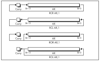
Interestingly, according to Intel’s i486 Microprocessor
Programmer’s Reference Manual, the 486 can RCR or
RCL a register by one bit in 3 cycles, but takes between 8
and 30 cycles to perform a multibit register RCR or
RCL!
No great lesson here, just a caution to be leery of multibit
RCR and RCL when performance matters—and to
take cycle-time documentation with a grain of salt.
Hardwired Far Jumps
Did you ever wonder how to code a far jump to an absolute address in
assembly language? Probably not, but if you ever do, you’re going to be
glad for this next item, because the obvious solution doesn’t work. You
might think all it would take to jump to, say, 1000:5 would be
JMP FAR PTR 1000:5, but you’d be wrong. That won’t even
assemble. You might then think to construct in memory a far pointer
containing 1000:5, as in the following:
Ptr dd ?
:
mov word ptr [Ptr],5
mov word ptr [Ptr+2],1000h
jmp [Ptr]That will work, but at a price in performance. On an 8088,
JMP DWORD PTR [*mem*] (an indirect far jump) takes at least
37 cycles; JMP DWORD PTR *label* (a direct far jump) takes
only 15 cycles (plus, almost certainly, some cycles for instruction
fetching). On a 386, an indirect far jump is documented to take at least
43 cycles in real mode (31 in protected mode); a direct far jump is
documented to take at least 12 cycles, about three times faster. In
truth, the difference between those two is nowhere near that big; the
fastest I’ve measured for a direct far jump is 21 cycles, and I’ve
measured indirect far jumps as fast as 30 cycles, so direct is still
faster, but not by so much. (Oh, those cycle-time documentation blues!)
Also, a direct far jump is documented to take at least 27 cycles in
protected mode; why the big difference in protected mode, I have no
idea.
At any rate, to return to our original problem of jumping to 1000:5: Although an indirect far jump will work, a direct far jump is still preferable.
Listing 9.7 shows a short program that performs a direct far call to
1000:5. (Don’t run it, unless you want to crash your system!) It does
this by creating a dummy segment at 1000H, so that the label
FarLabel can be created with the desired far attribute at
the proper location. (Segments created with “AT” don’t cause the
generation of any actual bytes or the allocation of any memory; they’re
just templates.) It’s a little kludgey, but at least it does work. There
may be a better solution; if you have one, pass it along.
LISTING 9.7 L9-7.ASM
; Program to perform a direct far jump to address 1000:5.
; *** Do not run this program! It's just an example of how ***
; *** to build a direct far jump to an absolute address ***
;
; Tested with TASM 2 and MASM 5.
FarSeg segment at 01000h
org 5
FarLabel label far
FarSeg ends
.model small
.code
start:
jmp FarLabel
end startBy the way, if you’re wondering how I figured this out, I merely applied my good friend Dan Illowsky’s long-standing rule for dealing with MASM:
If the obvious doesn’t work (and it usually doesn’t), just try everything you can think of, no matter how ridiculous, until you find something that does—a rule with plenty of history on its side.
Setting 32-Bit Registers: Time versus Space
To finish up this chapter, consider these two items. First, in 32-bit protected mode,
sub eax,eax
inc eaxtakes 4 cycles to execute, but is only 3 bytes long, while
mov eax,1takes only 2 cycles to execute, but is 5 bytes long (because native
mode constants are dwords and the MOV instruction doesn’t
sign-extend). Both code fragments are ways to set EAX to 1
(although the first affects the flags and the second doesn’t); this is a
classic trade-off of speed for space. Second,
or ebx,-1takes 2 cycles to execute and is 3 bytes long, while
move bx,-1takes 2 cycles to execute and is 5 bytes long. Both instructions set
EBX to -1; this is a classic trade-off of—gee, it’s not a
trade-off at all, is it? OR is a better way to set a 32-bit
register to all 1-bits, just as SUB or XOR is
a better way to set a register to all 0-bits. Who woulda thunk it? Just
goes to show how the 32-bit displacements and constants of 386 native
mode change the familiar landscape of 80x86 optimization.
Be warned, though, that I’ve found OR, AND,
ADD, and the like to be a cycle slower than
MOV when working with immediate operands on the 386 under
some circumstances, for reasons that thus far escape me. This just
reinforces the first rule of optimization: Measure your code in action,
and place not your trust in documented cycle times.
Chapter 10 – Patient Coding, Faster Code
How Working Quickly Can Bring Execution to a Crawl
My grandfather does The New York Times crossword puzzle every Sunday. In ink. With nary a blemish.
The relevance of which will become apparent in a trice.
What my grandfather is, is a pattern matcher par excellence. You’re a pattern matcher, too. So am I. We can’t help it; it comes with the territory. Try focusing on text and not reading it. Can’t do it. Can you hear the voice of someone you know and not recognize it? I can’t. And how in the Nine Billion Names of God is it that we’re capable of instantly recognizing one face out of the thousands we’ve seen in our lifetimes—even years later, from a different angle and in different light? Although we take them for granted, our pattern-matching capabilities are surely a miracle on the order of loaves and fishes.
By “pattern matching,” I mean more than just recognition, though. I mean that we are generally able to take complex and often seemingly woefully inadequate data, instantaneously match it in an incredibly flexible way to our past experience, extrapolate, and reach amazing conclusions, something that computers can scarcely do at all. Crossword puzzles are an excellent example; given a couple of letters and a cryptic clue, we’re somehow able to come up with one out of several hundred thousand words that we know. Try writing a program to do that! What’s more, we don’t process data in the serial brute-force way that computers do. Solutions tend to be virtually instantaneous or not at all; none of those “N log N” or “N2” execution times for us.
It goes without saying that pattern matching is good; more than that, it’s a large part of what we are, and, generally, the faster we are at it, the better. Not always, though. Sometimes insufficient information really is insufficient, and, in our haste to get the heady rush of coming up with a solution, incorrect or less-than-optimal conclusions are reached, as anyone who has ever done the Times Sunday crossword will attest. Still, my grandfather does that puzzle every Sunday in ink. What’s his secret? Patience and discipline. He never fills a word in until he’s confirmed it in his head via intersecting words, no matter how strong the urge may be to put something down where he can see it and feel like he’s getting somewhere.
There’s a surprisingly close parallel to programming here. Programming is certainly a sort of pattern matching in the sense I’ve described above, and, as with crossword puzzles, following your programming instincts too quickly can be a liability. For many programmers, myself included, there’s a strong urge to find a workable approach to a particular problem and start coding it right now, what some people call “hacking” a program. Going with the first thing your programming pattern matcher comes up with can be a lot of fun; there’s instant gratification and a feeling of unbounded creativity. Personally, I’ve always hungered to get results from my work as soon as possible; I gravitated toward graphics for its instant and very visible gratification. Over time, however, I’ve learned patience.
In this chapter, I’m going to walk you through a simple but illustrative case history that nicely points up the wisdom of delaying gratification when faced with programming problems, so that your mind has time to chew on the problems from other angles. The alternative solutions you find by doing this may seem obvious, once you’ve come up with them. They may not even differ greatly from your initial solutions. Often, however, they will be much better—and you’ll never even have the chance to decide whether they’re better or not if you take the first thing that comes into your head and run with it.
The Case for Delayed Gratification
Once upon a time, I set out to read Algorithms, by Robert Sedgewick (Addison-Wesley), which turned out to be a wonderful, stimulating, and most useful book, one that I recommend highly. My story, however, involves only what happened in the first 12 pages, for it was in those pages that Sedgewick discussed Euclid’s algorithm.
Euclid’s algorithm (discovered by Euclid, of Euclidean geometry fame, a very long time ago, way back when computers still used core memory) is a straightforward algorithm that solves one of the simplest problems imaginable: finding the greatest common integer divisor (GCD) of two positive integers. Sedgewick points out that this is useful for reducing a fraction to its lowest terms. I’m sure it’s useful for other things, as well, although none spring to mind. (A long time ago, I wrote an article about optimizing a bit of code that wasn’t even vaguely time-critical, and got swamped with letters telling me so. I knew it wasn’t time-critical; it was just a good example. So for now, close your eyes and imagine that finding the GCD is not only necessary but must also be done as quickly as possible, because it’s perfect for the point I want to make here and now. Okay?)
The problem at hand, then, is simply this: Find the largest integer value that evenly divides two arbitrary positive integers. That’s all there is to it. So warm up your pattern matchers…and go!
The Brute-Force Syndrome
I have a funny feeling that you’d already figured out how to find the GCD before I even said “go.” That’s what I did when reading Algorithms; before I read another word, I had to figure it out for myself. Programmers are like that; give them a problem and their eyes immediately glaze over as they try to solve it before you’ve even shut your mouth. That sort of instant response can certainly be impressive, but it can backfire, too, as it did in my case.
You see, I fell victim to a common programming pitfall, the “brute-force” syndrome. The basis of this syndrome is that there are many problems that have obvious, brute-force solutions—with one small drawback. The drawback is that if you were to try to apply a brute-force solution by hand—that is, work a single problem out with pencil and paper or a calculator—it would generally require that you have the patience and discipline to work on the problem for approximately seven hundred years, not counting eating and sleeping, in order to get an answer. Finding all the prime numbers less than 1,000,000 is a good example; just divide each number up to 1,000,000 by every lesser number, and see what’s left standing. For most of the history of humankind, people were forced to think of cleverer solutions, such as the Sieve of Eratosthenes (we’d have been in big trouble if the ancient Greeks had had computers), mainly because after about five minutes of brute force-type work, people’s attention gets diverted to other important matters, such as how far a paper airplane will fly from a second-story window.
Not so nowadays, though. Computers love boring work; they’re very patient and disciplined, and, besides, one human year = seven dog years = two zillion computer years. So when we’re faced with a problem that has an obvious but exceedingly lengthy solution, we’re apt to say, “Ah, let the computer do that, it’s fast,” and go back to making paper airplanes. Unfortunately, brute-force solutions tend to be slow even when performed by modern-day microcomputers, which are capable of several MIPS except when I’m late for an appointment and want to finish a compile and run just one more test before I leave, in which case the crystal in my computer is apparently designed to automatically revert to 1 Hz.)
The solution that I instantly came up with to finding the GCD is about as brute- force as you can get: Divide both the larger integer (iL) and the smaller integer (iS) by every integer equal to or less than the smaller integer, until a number is found that divides both evenly, as shown in Figure 10.1. This works, but it’s a lousy solution, requiring as many as iS*2 divisions; very expensive, especially for large values of iS. For example, finding the GCD of 30,001 and 30,002 would require 60,002 divisions, which alone, disregarding tests and branches, would take about 2 seconds on an 8088, and more than 50 milliseconds even on a 25 MHz 486—a very long time in computer years, and not insignificant in human years either.
Listing 10.1 is an implementation of the brute-force approach to GCD calculation. Table 10.1 shows how long it takes this approach to find the GCD for several integer pairs. As expected, performance is extremely poor when iS is large.
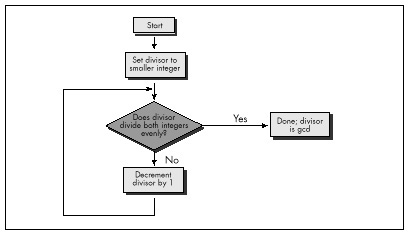
Integer pairs for which to find GCD
| 90 & 27 | 42 & 998 | 453 & 121 | 27432 & 165 | 27432 & 17550 | |
|---|---|---|---|---|---|
| Listing 10.1 (Brute force) | 60µs (100%) | 110µs (100%) | 311ms (100%) | 426µs (100%) | 43580µs (100%) |
| Listing 10.2 (Subtraction) | 25 (42%) | 72 (65%) | 67 (22%) | 280 (66%) | 72 (0.16%) |
| Listing 10.3 (Division: code recursive Euclid’s algorithm) | 20 (33%) | 33 (30%) | 48 (15%) | 32 (8%) | 53 (0.12%) |
| Listing 10.4 (C version of data recursive Euclid’s algorithm; normal optimization) | 12 (20%) | 17 (15%) | 25 (8%) | 16 (4%) | 26 (0.06%) |
| Listing 10.4 (/Ox = maximumoptimization) | 12 (20%) | 16 (15%) | 20 (6%) | 15 (4%) | 23 (0.05%) |
| Listing 10.5 (Assembly version of data recursive Euclid’s algorithm) | 10 (17%) | 10 (9%) | 15 (5%) | 10 (2%) | 17 (0.04%) |
Note: Performance of Listings 10.1 through 10.5 in finding the greatest common divisors of various pairs of integers. Times are in microseconds. Percentages represent execution time as a percentage of the execution time of Listing 10.1 for the same integer pair. Listings 10.1-10.4 were compiled with Microsoft C /C++ except as noted, the default optimization was used. All times measured with the Zen timer (from Chapter 3) on a 20 MHz cached 386.
LISTING 10.1 L10-1.C
/* Finds and returns the greatest common divisor of two positive
integers. Works by trying every integral divisor between the
smaller of the two integers and 1, until a divisor that divides
both integers evenly is found. All C code tested with Microsoft
and Borland compilers.*/
unsigned int gcd(unsigned int int1, unsigned int int2) {
unsigned int temp, trial_divisor;
/* Swap if necessary to make sure that int1 >= int2 */
if (int1 < int2) {
temp = int1;
int1 = int2;
int2 = temp;
}
/* Now just try every divisor from int2 on down, until a common
divisor is found. This can never be an infinite loop because
1 divides everything evenly */
for (trial_divisor = int2; ((int1 % trial_divisor) != 0) ||
((int2 % trial_divisor) != 0); trial_divisor—)
;
return(trial_divisor);
}Wasted Breakthroughs
Sedgewick’s first solution to the GCD problem was pretty much the one I came up with. He then pointed out that the GCD of iL and iS is the same as the GCD of iL-iS and iS. This was obvious (once Sedgewick pointed it out); by the very nature of division, any number that divides iL evenly nL times and iS evenly nS times must divide iL-iS evenly nL-nS times. Given that insight, I immediately designed a new, faster approach, shown in Listing 10.2.
LISTING 10.2 L10-2.C
/* Finds and returns the greatest common divisor of two positive
integers. Works by subtracting the smaller integer from the
larger integer until either the values match (in which case
that's the gcd), or the larger integer becomes the smaller of
the two, in which case the two integers swap roles and the
subtraction process continues. */
unsigned int gcd(unsigned int int1, unsigned int int2) {
unsigned int temp;
/* If the two integers are the same, that's the gcd and we're
done */
if (int1 == int2) {
return(int1);
}
/* Swap if necessary to make sure that int1 >= int2 */
if (int1 < int2) {
temp = int1;
int1 = int2;
int2 = temp;
}
/* Subtract int2 from int1 until int1 is no longer the larger of
the two */
do {
int1 -= int2;
} while (int1 > int2);
/* Now recursively call this function to continue the process */
return(gcd(int1, int2));
}Listing 10.2 repeatedly subtracts iS from iL until iL becomes less than or equal to iS. If iL becomes equal to iS, then that’s the GCD; alternatively, if iL becomes less than iS, iL and iS switch values, and the process is repeated, as shown in Figure 10.2. The number of iterations this approach requires relative to Listing 10.1 depends heavily on the values of iL and iS, so it’s not always faster, but, as Table 10.1 indicates, Listing 10.2 is generally much better code.
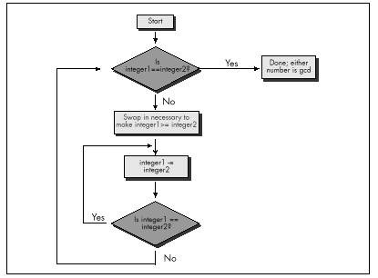
Listing 10.2 is a far graver misstep than Listing 10.1, for all that it’s faster. Listing 10.1 is obviously a hacked-up, brute-force approach; no one could mistake it for anything else. It could be speeded up in any of a number of ways with a little thought. (Simply skipping testing all the divisors between iS and iS/2, not inclusive, would cut the worst-case time in half, for example; that’s not a particularly good optimization, but it illustrates how easily Listing 10.1 can be improved.) Listing 10.1 is a hack job, crying out for inspiration.
Listing 10.2, on the other hand, has gotten the inspiration—and largely wasted it through haste. Had Sedgewick not told me otherwise, I might well have assumed that Listing 10.2 was optimized, a mistake I would never have made with Listing 10.1. I experienced a conceptual breakthrough when I understood Sedgewick’s point: A smaller number can be subtracted from a larger number without affecting their GCD, thereby inexpensively reducing the scale of the problem. And, in my hurry to make this breakthrough reality, I missed its full scope. As Sedgewick says on the very next page, the number that one gets by subtracting iS from iL until iL is less than iS is precisely the same as the remainder that one gets by dividing iL by iS—again, this is inherent in the nature of division—and that is the basis for Euclid’s algorithm, shown in Figure 10.3. Listing 10.3 is an implementation of Euclid’s algorithm.
LISTING 10.3 L10-3.C
/* Finds and returns the greatest common divisor of two integers.
Uses Euclid's algorithm: divides the larger integer by the
smaller; if the remainder is 0, the smaller integer is the GCD,
otherwise the smaller integer becomes the larger integer, the
remainder becomes the smaller integer, and the process is
repeated. */
static unsigned int gcd_recurs(unsigned int, unsigned int);
unsigned int gcd(unsigned int int1, unsigned int int2) {
unsigned int temp;
/* If the two integers are the same, that's the GCD and we're
done */
if (int1 == int2) {
return(int1);
}
/* Swap if necessary to make sure that int1 >= int2 */
if (int1 < int2) {
temp = int1;
int1 = int2;
int2 = temp;
}
/* Now call the recursive form of the function, which assumes
that the first parameter is the larger of the two */
return(gcd_recurs(int1, int2));
}
static unsigned int gcd_recurs(unsigned int larger_int,
unsigned int smaller_int)
{
int temp;
/* If the remainder of larger_int divided by smaller_int is 0,
then smaller_int is the gcd */
if ((temp = larger_int % smaller_int) == 0) {
return(smaller_int);
}
/* Make smaller_int the larger integer and the remainder the
smaller integer, and call this function recursively to
continue the process */
return(gcd_recurs(smaller_int, temp));
}As you can see from Table 10.1, Euclid’s algorithm is superior, especially for large numbers (and imagine if we were working with large longs!).
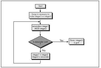
Give your mind time and space to wander around the edges of important programming problems before you settle on any one approach. I titled this book’s first chapter “The Best Optimizer Is between Your Ears,” and that’s still true; what’s even more true is that the optimizer between your ears does its best work not at the implementation stage, but at the very beginning, when you try to imagine how what you want to do and what a computer is capable of doing can best be brought together.
Recursion
Euclid’s algorithm lends itself to recursion beautifully, so much so that an implementation like Listing 10.3 comes almost without thought. Again, though, take a moment to stop and consider what’s really going on, at the assembly language level, in Listing 10.3. There’s recursion and then there’s recursion; code recursion and data recursion, to be exact. Listing 10.3 is code recursion—recursion through calls—the sort most often used because it is conceptually simplest. However, code recursion tends to be slow because it pushes parameters and calls a subroutine for every iteration. Listing 10.4, which uses data recursion, is much faster and no more complicated than Listing 10.3. Actually, you could just say that Listing 10.4 uses a loop and ignore any mention of recursion; conceptually, though, Listing 10.4 performs the same recursive operations that Listing 10.3 does.
LISTING 10.4 L10-4.C
/* Finds and returns the greatest common divisor of two integers.
Uses Euclid's algorithm: divides the larger integer by the
smaller; if the remainder is 0, the smaller integer is the GCD,
otherwise the smaller integer becomes the larger integer, the
remainder becomes the smaller integer, and the process is
repeated. Avoids code recursion. */
unsigned int gcd(unsigned int int1, unsigned int int2) {
unsigned int temp;
/* Swap if necessary to make sure that int1 >= int2 */
if (int1 < int2) {
temp = int1;
int1 = int2;
int2 = temp;
}
/* Now loop, dividing int1 by int2 and checking the remainder,
until the remainder is 0. At each step, if the remainder isn't
0, assign int2 to int1, and the remainder to int2, then
repeat */
for (;;) {
/* If the remainder of int1 divided by int2 is 0, then int2 is
the gcd */
if ((temp = int1 % int2) == 0) {
return(int2);
}
/* Make int2 the larger integer and the remainder the
smaller integer, and repeat the process */
int1 = int2;
int2 = temp;
}
}Patient Optimization
At long last, we’re ready to optimize GCD determination in the classic sense. Table 10.1 shows the performance of Listing 10.4 with and without Microsoft C/C++’s maximum optimization, and also shows the performance of Listing 10.5, an assembly language version of Listing 10.4. Sure, the optimized versions are faster than the unoptimized version of Listing 10.4—but the gains are small compared to those realized from the higher-level optimizations in Listings 10.2 through 10.4.
LISTING 10.5 L10-5.ASM
; Finds and returns the greatest common divisor of two integers.
; Uses Euclid's algorithm: divides the larger integer by the
; smaller; if the remainder is 0, the smaller integer is the GCD,
; otherwise the smaller integer becomes the larger integer, the
; remainder becomes the smaller integer, and the process is
; repeated. Avoids code recursion.
;
;
;
; C near-callable as:
; unsigned int gcd(unsigned int int1, unsigned int int2);
; Parameter structure:
parms struc
dw ? ;pushed BP
dw ? ;pushed return address
int1 dw ? ;integers for which to find
int2 dw ? ; the GCD
parms ends
.model small
.code
public _gcd
align 2
_gcd proc near
push bp ;preserve caller's stack frame
mov bp,sp ;set up our stack frame
push si ;preserve caller's register variables
push di
;Swap if necessary to make sure that int1 >= int2
mov ax,int1[bp]
mov bx,int2[bp]
cmp ax,bx ;is int1 >= int2?
jnb IntsSet ;yes, so we're all set
xchg ax,bx ;no, so swap int1 and int2
IntsSet:
; Now loop, dividing int1 by int2 and checking the remainder, until
; the remainder is 0. At each step, if the remainder isn't 0, assign
; int2 to int1, and the remainder to int2, then repeat.
GCDLoop:
;if the remainder of int1 divided by
; int2 is 0, then int2 is the gcd
sub dx,dx ;prepare int1 in DX:AX for division
div bx ;int1/int2; remainder is in DX
and dx,dx ;is the remainder zero?
jz Done ;yes, so int2 (BX) is the gcd
;no, so move int2 to int1 and the
; remainder to int2, and repeat the
; process
mov ax,bx ;int1 = int2;
mov bx,dx ;int2 = remainder from DIV
;—start of loop unrolling; the above is repeated three times—
sub dx,dx ;prepare int1 in DX:AX for division
div bx ;int1/int2; remainder is in DX
and dx,dx ;is the remainder zero?
jz Done ;yes, so int2 (BX) is the gcd
mov ax,bx ;int1 = int2;
mov bx,dx ;int2 = remainder from DIV
;—
sub dx,dx ;prepare int1 in DX:AX for division
div bx ;int1/int2; remainder is in DX
and dx,dx ;is the remainder zero?
jz Done ;yes, so int2 (BX) is the gcd
mov ax,bx ;int1 = int2;
mov bx,dx ;int2 = remainder from DIV
;—
sub dx,dx ;prepare int1 in DX:AX for division
div bx ;int1/int2; remainder is in DX
and dx,dx ;is the remainder zero?
jz Done ;yes, so int2 (BX) is the gcd
mov ax,bx ;int1 = int2;
mov bx,dx ;int2 = remainder from DIV
;—end of loop unrolling—
jmp GCDLoop
align2
Done:
mov ax,bx ;return the GCD
pop di ;restore caller's register variables
pop si
pop bp ;restore caller's stack frame
ret
_gcd endp
endAssembly language optimization is pattern matching on a local scale. Frankly, it’s also the sort of boring, brute-force work that people are lousy at; compilers could out-optimize you at this level with one pass tied behind their back if they knew as much about the code you’re writing as you do, which they don’t.
Computers are much worse at that sort of pattern matching than humans; computers have no way to integrate vast amounts of disparate information, much of it only vaguely defined or subject to change. People, oddly enough, are better at global optimization than at local optimization. For one thing, it’s more interesting. For another, it’s complex and imprecise enough to allow intuition and inspiration, two vastly underrated programming tools, to come to the fore. And, as I pointed out earlier, people tend to perform instantaneous solutions to even the most complex problems, while computers bog down in geometrically or exponentially increasing execution times. Oh, it may take days or weeks for a person to absorb enough information to be able to reach a solution, and the solution may only be near-optimal—but the solution itself (or, at least, each of the pieces of the solution) arrives in a flash.
Those flashes are your programming pattern matcher doing its job. Your job is to give your pattern matcher the opportunity to get to know each problem and run through it two or three times, from different angles, to see what unexpected solutions it can come up with.
Pull back the reins a little. Don’t measure progress by lines of code written today; measure it instead by overall progress and by quality. Relax and listen to that quiet inner voice that provides the real breakthroughs. Stop, look, listen—and think. Not only will you find that it’s a more productive and creative way to program—but you’ll also find that it’s more fun.
And think what you could do with all those extra computer years!
Chapter 11 – Pushing the 286 and 386
New Registers, New Instructions, New Timings, New Complications
This chapter, adapted from my earlier book Zen of Assembly Language (1989; now out of print), provides an overview of the 286 and 386, often contrasting those processors with the 8088. At the time I originally wrote this, the 8088 was the king of processors, and the 286 and 386 were the new kids on the block. Today, of course, all three processors are past their primes, but many millions of each are still in use, and the 386 in particular is still well worth considering when optimizing software.
This chapter provides an interesting look at the evolution of the x86 architecture, to a greater degree than you might expect, for the x86 family came into full maturity with the 386; the 486 and the Pentium are really nothing more than faster 386s, with very little in the way of new functionality. In contrast, the 286 added a number of instructions, respectable performance, and protected mode to the 8088’s capabilities, and the 386 added more instructions and a whole new set of addressing modes, and brought the x86 family into the 32-bit world that represents the future (and, increasingly, the present) of personal computing. This chapter also provides insight into the effects on optimization of the variations in processors and memory architectures that are common in the PC world. So, although the 286 and 386 no longer represent the mainstream of computing, this chapter is a useful mix of history lesson, x86 overview, and details on two workhorse processors that are still in wide use.
Family Matters
While the x86 family is a large one, only a few members of the family—which includes the 8088, 8086, 80188, 80186, 286, 386SX, 386DX, numerous permutations of the 486, and now the Pentium—really matter.
The 8088 is now all but extinct in the PC arena. The 8086 was used fairly widely for a while, but has now all but disappeared. The 80186 and 80188 never really caught on for use in PC and don’t require further discussion.
That leaves us with the high-end chips: the 286, the 386SX, the 386, the 486, and the Pentium. At this writing, the 386SX is fast going the way of the 8088; people are realizing that its relatively small cost advantage over the 386 isn’t enough to offset its relatively large performance disadvantage. After all, the 386SX suffers from the same debilitating problem that looms over the 8088—a too-small bus. Internally, the 386SX is a 32-bit processor, but externally, it’s a 16-bit processor, a non-optimal architecture, especially for 32-bit code.
I’m not going to discuss the 386SX in detail. If you do find yourself programming for the 386SX, follow the same general rules you should follow for the 8088: use short instructions, use the registers as heavily as possible, and don’t branch. In other words, avoid memory, since the 386SX is by definition better at processing data internally than it is at accessing memory.
The 486 is a world unto itself for the purposes of optimization, and the Pentium is a universe unto itself. We’ll treat them separately in later chapters.
This leaves us with just two processors: the 286 and the 386. Each was the PC standard in its day. The 286 is no longer used in new systems, but there are millions of 286-based systems still in daily use. The 386 is still being used in new systems, although it’s on the downhill leg of its lifespan, and it is in even wider use than the 286. The future clearly belongs to the 486 and Pentium, but the 286 and 386 are still very much a part of the present-day landscape.
Crossing the Gulf to the 286 and the 386
Apart from vastly improved performance, the biggest difference between the 8088 and the 286 and 386 (as well as the later Intel CPUs) is that the 286 introduced protected mode, and the 386 greatly expanded the capabilities of protected mode. We’re only going to talk about real-mode operation of the 286 and 386 in this book, however. Protected mode offers a whole new memory management scheme, one that isn’t supported by the 8088. Only code specifically written for protected mode can run in that mode; it’s an alien and hostile environment for MS-DOS programs.
In particular, segments are different creatures in protected mode. They’re selectors—indexes into a table of segment descriptors—rather than plain old registers, and can’t be set to arbitrary values. That means that segments can’t be used for temporary storage or as part of a fast indivisible 32-bit load from memory, as in
les ax,dword ptr [LongVar]
mov dx,eswhich loads LongVar into DX:AX faster than this:
mov ax,word ptr [LongVar]
mov dx,word ptr [LongVar+2]Protected mode uses those altered segment registers to offer access to a great deal more memory than real mode: The 286 supports 16 megabytes of memory, while the 386 supports 4 gigabytes (4K megabytes) of physical memory and 64 terabytes (64K gigabytes!) of virtual memory.
In protected mode, your programs generally run under an operating system (OS/2, Unix, Windows NT or the like) that exerts much more control over the computer than does MS-DOS. Protected mode operating systems can generally run multiple programs simultaneously, and the performance of any one program may depend far less on code quality than on how efficiently the program uses operating system services and how often and under what circumstances the operating system preempts the program. Protected mode programs are often mostly collections of operating system calls, and the performance of whatever code isn’t operating-system oriented may depend primarily on how large a time slice the operating system gives that code to run in.
In short, taken as a whole, protected mode programming is a different kettle of fish altogether from what I’ve been describing in this book. There’s certainly a knack to optimizing specifically for protected mode under a given operating system…but it’s not what we’ve been learning, and now is not the time to pursue it further. In general, though, the optimization strategies discussed in this book still hold true in protected mode; it’s just issues specific to protected mode or a particular operating system that we won’t discuss.
In the Lair of the Cycle-Eaters, Part II
Under the programming interface, the 286 and 386 differ considerably from the 8088. Nonetheless, with one exception and one addition, the cycle-eaters remain much the same on computers built around the 286 and 386. Next, we’ll review each of the familiar cycle-eaters I covered in Chapter 4 as they apply to the 286 and 386, and we’ll look at the new member of the gang, the data alignment cycle-eater.
The one cycle-eater that vanishes on the 286 and 386 is the 8-bit bus cycle-eater. The 286 is a 16-bit processor both internally and externally, and the 386 is a 32-bit processor both internally and externally, so the Execution Unit/Bus Interface Unit size mismatch that plagues the 8088 is eliminated. Consequently, there’s no longer any need to use byte-sized memory variables in preference to word-sized variables, at least so long as word-sized variables start at even addresses, as we’ll see shortly. On the other hand, access to byte-sized variables still isn’t any slower than access to word-sized variables, so you can use whichever size suits a given task best.
You might think that the elimination of the 8-bit bus cycle-eater would mean that the prefetch queue cycle-eater would also vanish, since on the 8088 the prefetch queue cycle-eater is a side effect of the 8-bit bus. That would seem all the more likely given that both the 286 and the 386 have larger prefetch queues than the 8088 (6 bytes for the 286, 16 bytes for the 386) and can perform memory accesses, including instruction fetches, in far fewer cycles than the 8088.
However, the prefetch queue cycle-eater doesn’t vanish on either the 286 or the 386, for several reasons. For one thing, branching instructions still empty the prefetch queue, so instruction fetching still slows things down after most branches; when the prefetch queue is empty, it doesn’t much matter how big it is. (Even apart from emptying the prefetch queue, branches aren’t particularly fast on the 286 or the 386, at a minimum of seven-plus cycles apiece. Avoid branching whenever possible.)
After a branch it does matter how fast the queue can refill, and there we come to the second reason the prefetch queue cycle-eater lives on: The 286 and 386 are so fast that sometimes the Execution Unit can execute instructions faster than they can be fetched, even though instruction fetching is much faster on the 286 and 386 than on the 8088.
(All other things being equal, too-slow instruction fetching is more of a problem on the 286 than on the 386, since the 386 fetches 4 instruction bytes at a time versus the 2 instruction bytes fetched per memory access by the 286. However, the 386 also typically runs at least twice as fast as the 286, meaning that the 386 can easily execute instructions faster than they can be fetched unless very high-speed memory is used.)
The most significant reason that the prefetch queue cycle-eater not only survives but prospers on the 286 and 386, however, lies in the various memory architectures used in computers built around the 286 and 386. Due to the memory architectures, the 8-bit bus cycle-eater is replaced by a new form of the wait state cycle-eater: wait states on accesses to normal system memory.
System Wait States
The 286 and 386 were designed to lose relatively little performance to the prefetch queue cycle-eater…when used with zero-wait-state memory: memory that can complete memory accesses so rapidly that no wait states are needed. However, true zero-wait-state memory is almost never used with those processors. Why? Because memory that can keep up with a 286 is fairly expensive, and memory that can keep up with a 386 is very expensive. Instead, computer designers use alternative memory architectures that offer more performance for the dollar—but less performance overall—than zero-wait-state memory. (It is possible to build zero-wait-state systems for the 286 and 386; it’s just so expensive that it’s rarely done.)
The IBM AT and true compatibles use one-wait-state memory (some AT clones use zero-wait-state memory, but such clones are less common than one-wait-state AT clones). The 386 systems use a wide variety of memory systems—including high-speed caches, interleaved memory, and static-column RAM—that insert anywhere from 0 to about 5 wait states (and many more if 8 or 16-bit memory expansion cards are used); the exact number of wait states inserted at any given time depends on the interaction between the code being executed and the memory system it’s running on.
The many memory systems in use make it impossible for us to optimize for 286/386 computers with the precision that’s possible on the 8088. Instead, we must write code that runs reasonably well under the varying conditions found in the 286/386 arena.
The wait states that occur on most accesses to system memory in 286 and 386 computers mean that nearly every access to system memory—memory in the DOS’s normal 640K memory area—is slowed down. (Accesses in computers with high-speed caches may be wait-state-free if the desired data is already in the cache, but will certainly encounter wait states if the data isn’t cached; this phenomenon produces highly variable instruction execution times.) While this is our first encounter with system memory wait states, we have run into a wait-state cycle-eater before: the display adapter cycle-eater, which we discussed along with the other 8088 cycle-eaters way back in Chapter 4. System memory generally has fewer wait states per access than display memory. However, system memory is also accessed far more often than display memory, so system memory wait states hurt plenty—and the place they hurt most is instruction fetching.
Consider this: The 286 can store an immediate value to memory, as in
MOV [WordVar],0, in just 3 cycles. However, that
instruction is 6 bytes long. The 286 is capable of fetching 1 word every
2 cycles; however, the one-wait-state architecture of the AT stretches
that to 3 cycles. Consequently, nine cycles are needed to fetch the six
instruction bytes. On top of that, 3 cycles are needed to write to
memory, bringing the total memory access time to 12 cycles. On balance,
memory access time—especially instruction prefetching—greatly exceeds
execution time, to the extent that this particular instruction can take
up to four times as long to run as it does to execute in the Execution
Unit.
And that, my friend, is unmistakably the prefetch queue cycle-eater. I might add that the prefetch queue cycle-eater is in rare good form in the above example: A 4-to-1 ratio of instruction fetch time to execution time is in a class with the best (or worst!) that’s found on the 8088.
Let’s check out the prefetch queue cycle-eater in action. Listing
11.1 times MOV [WordVar],0. The Zen timer reports that on a
one-wait-state 10 MHz 286-based AT clone (the computer used for all
tests in this chapter), Listing 11.1 runs in 1.27 µs per instruction.
That’s 12.7 cycles per instruction, just as we calculated. (That extra
seven-tenths of a cycle comes from DRAM refresh, which we’ll get to
shortly.)
LISTING 11.1 L11-1.ASM
;
; *** Listing 11.1 ***
;
; Measures the performance of an immediate move to
; memory, in order to demonstrate that the prefetch
; queue cycle-eater is alive and well on the AT.
;
jmp Skip
;
even ;always make sure word-sized memory
; variables are word-aligned!
WordVar dw 0
;
Skip:
call ZTimerOn
rept 1000
mov [WordVar],0
endm
call ZTimerOffWhat does this mean? It means that, practically speaking, the 286 as used in the AT doesn’t have a 16-bit bus. From a performance perspective, the 286 in an AT has two-thirds of a 16-bit bus (a 10.7-bit bus?), since every bus access on an AT takes 50 percent longer than it should. A 286 running at 10 MHz should be able to access memory at a maximum rate of 1 word every 200 ns; in a 10 MHz AT, however, that rate is reduced to 1 word every 300 ns by the one-wait-state memory.
In short, a close relative of our old friend the 8-bit bus cycle-eater—the system memory wait state cycle-eater—haunts us still on all but zero-wait-state 286 and 386 computers, and that means that the prefetch queue cycle-eater is alive and well. (The system memory wait state cycle-eater isn’t really a new cycle-eater, but rather a variant of the general wait state cycle-eater, of which the display adapter cycle-eater is yet another variant.) While the 286 in the AT can fetch instructions much faster than can the 8088 in the PC, it can execute those instructions faster still.
The picture is less clear in the 386 world since there are so many different memory architectures, but similar problems can occur in any computer built around a 286 or 386. The prefetch queue cycle-eater is even a factor—albeit a lesser one—on zero-wait-state machines, both because branching empties the queue and because some instructions can outrun even zero—5 cycles longer than the official execution time.)
To summarize:
- Memory-accessing instructions don’t run at their official speeds on non-zero-wait-state 286/386 computers.
- The prefetch queue cycle-eater reduces performance on 286/386 computers, particularly when non-zero-wait-state memory is used.
- Branches often execute at less than their rated speeds on the 286 and 386 since the prefetch queue is emptied.
- The extent to which the prefetch queue and wait states affect performance varies from one 286/386 computer to another, making precise optimization impossible.
What’s to be learned from all this? Several things:
- Keep your instructions short.
- Keep it in the registers; avoid memory, since memory generally can’t keep up with the processor.
- Don’t jump.
Of course, those are exactly the rules that apply to 8088 optimization as well. Isn’t it convenient that the same general rules apply across the board?
Data Alignment
Thanks to its 16-bit bus, the 286 can access word-sized memory variables just as fast as byte-sized variables. There’s a catch, however: That’s only true for word-sized variables that start at even addresses. When the 286 is asked to perform a word-sized access starting at an odd address, it actually performs two separate accesses, each of which fetches 1 byte, just as the 8088 does for all word-sized accesses.
Figure 11.1 illustrates this phenomenon. The conversion of word-sized accesses to odd addresses into double byte-sized accesses is transparent to memory-accessing instructions; all any instruction knows is that the requested word has been accessed, no matter whether 1 word-sized access or 2 byte-sized accesses were required to accomplish it.
The penalty for performing a word-sized access starting at an odd address is easy to calculate: Two accesses take twice as long as one access.
That, in a nutshell, is the data alignment cycle-eater, the one new cycle-eater of the 286 and 386. (The data alignment cycle-eater is a close relative of the 8088’s 8-bit bus cycle-eater, but since it behaves differently—occurring only at odd addresses—and is avoided with a different workaround, we’ll consider it to be a new cycle-eater.)
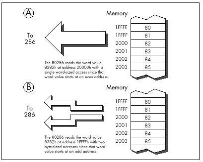
The way to deal with the data alignment cycle-eater is
straightforward: Don’t perform word-sized accesses to odd addresses
on the 286 if you can help it. The easiest way to avoid the data
alignment cycle-eater is to place the directive EVEN before
each of your word-sized variables. EVEN forces the offset
of the next byte assembled to be even by inserting a NOP if
the current offset is odd; consequently, you can ensure that any
word-sized variable can be accessed efficiently by the 286 simply by
preceding it with EVEN.
Listing 11.2, which accesses memory a word at a time with each word
starting at an odd address, runs on a 10 MHz AT clone in 1.27 ms per
repetition of MOVSW, or 0.64 ms per word-sized memory
access. That’s 6-plus cycles per word-sized access, which breaks down to
two separate memory accesses—3 cycles to access the high byte of each
word and 3 cycles to access the low byte of each word, the inevitable
result of non-word-aligned word-sized memory accesses—plus a bit extra
for DRAM refresh.
LISTING 11.2 L11-2.ASM
;
; *** Listing 11.2 ***
;
; Measures the performance of accesses to word-sized
; variables that start at odd addresses (are not
; word-aligned).
;
Skip:
push ds
pop es
mov si,1 ;source and destination are the same
mov di,si ; and both are not word-aligned
mov cx,1000 ;move 1000 words
cld
call ZTimerOn
rep movsw
call ZTimerOffOn the other hand, Listing 11.3, which is exactly the same as Listing
11.2 save that the memory accesses are word-aligned (start at even
addresses), runs in 0.64 ms per repetition of MOVSW, or
0.32 µs per word-sized memory access. That’s 3 cycles per word-sized
access—exactly twice as fast as the non-word-aligned accesses of Listing
11.2, just as we predicted.
LISTING 11.3 L11-3.ASM
;
; *** Listing 11.3 ***
;
; Measures the performance of accesses to word-sized
; variables that start at even addresses (are word-aligned).
;
Skip:
push ds
pop es
sub si,si ;source and destination are the same
mov di,si ; and both are word-aligned
mov cx,1000 ;move 1000 words
cld
call ZTimerOn
rep movsw
call ZTimerOffThe data alignment cycle-eater has intriguing implications for speeding up 286/386 code. The expenditure of a little care and a few bytes to make sure that word-sized variables and memory blocks are word-aligned can literally double the performance of certain code running on the 286. Even if it doesn’t double performance, word alignment usually helps and never hurts.
Code Alignment
Lack of word alignment can also interfere with instruction fetching on the 286, although not to the extent that it interferes with access to word-sized memory variables. The 286 prefetches instructions a word at a time; even if a given instruction doesn’t begin at an even address, the 286 simply fetches the first byte of that instruction at the same time that it fetches the last byte of the previous instruction, as shown in Figure 11.2, then separates the bytes internally. That means that in most cases, instructions run just as fast whether they’re word-aligned or not.
There is, however, a non-word-alignment penalty on branches to odd addresses. On a branch to an odd address, the 286 is only able to fetch 1 useful byte with the first instruction fetch following the branch, as shown in Figure 11.3. In other words, lack of word alignment of the target instruction for any branch effectively cuts the instruction-fetching power of the 286 in half for the first instruction fetch after that branch. While that may not sound like much, you’d be surprised at what it can do to tight loops; in fact, a brief story is in order.
When I was developing the Zen timer, I used my trusty 10 MHz 286-based AT clone to verify the basic functionality of the timer by measuring the performance of simple instruction sequences. I was cruising along with no problems until I timed the following code:
mov cx,1000
call ZTimerOn
LoopTop:
loop LoopTop
call ZTimerOff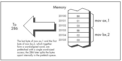
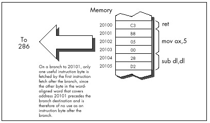
Now, this code should run in, say, about 12 cycles per loop
at most. Instead, it took over 14 cycles per loop, an execution time
that I could not explain in any way. After rolling it around in my head
for a while, I took a look at the code under a debugger…and the answer
leaped out at me. The loop began at an odd address! That meant
that two instruction fetches were required each time through the loop;
one to get the opcode byte of the LOOP instruction, which
resided at the end of one word-aligned word, and another to get the
displacement byte, which resided at the start of the next word-aligned
word.
One simple change brought the execution time down to a reasonable 12.5 cycles per loop:
mov cx,1000
call ZTimerOn
even
LoopTop:
loop LoopTop
call ZTimerOffWhile word-aligning branch destinations can improve branching
performance, it’s a nuisance and can increase code size a good deal, so
it’s not worth doing in most code. Besides, EVEN inserts a
NOP instruction if necessary, and the time required to
execute a NOP can sometimes cancel the performance
advantage of having a word-aligned branch destination.
I recommend that you only go out of your way to word-align the start offsets of your subroutines, as in:
even
FindChar proc near
:In my experience, this simple practice is the one form of code alignment that consistently provides a reasonable return for bytes and effort expended, although sometimes it also pays to word-align tight time-critical loops.
Alignment and the 386
So far we’ve only discussed alignment as it pertains to the 286. What, you may well ask, of the 386?
The 386 adds the issue of doubleword alignment (that is, alignment to addresses that are multiples of four.) The rule for the 386 is: Word-sized memory accesses should be word-aligned (it’s impossible for word-aligned word-sized accesses to cross doubleword boundaries), and doubleword-sized memory accesses should be doubleword-aligned. However, in real (as opposed to 32-bit protected) mode, doubleword-sized memory accesses are rare, so the simple word-alignment rule we’ve developed for the 286 serves for the 386 in real mode as well.
As for code alignment…the subroutine-start word-alignment rule of the 286 serves reasonably well there too since it avoids the worst case, where just 1 byte is fetched on entry to a subroutine. While optimum performance would dictate doubleword alignment of subroutines, that takes 3 bytes, a high price to pay for an optimization that improves performance only on the post 286 processors.
Alignment and the Stack
One side-effect of the data alignment cycle-eater of the 286 and 386
is that you should never allow the stack pointer to become odd.
(You can make the stack pointer odd by adding an odd value to it or
subtracting an odd value from it, or by loading it with an odd value.)
An odd stack pointer on the 286 or 386 (or a non-doubleword-aligned
stack in 32-bit protected mode on the 386, 486, or Pentium) will
significantly reduce the performance of PUSH,
POP, CALL, and RET, as well as
INT and IRET, which are executed to invoke DOS
and BIOS functions, handle keystrokes and incoming serial characters,
and manage the mouse. I know of a Forth programmer who vastly improved
the performance of a complex application on the AT simply by forcing the
Forth interpreter to maintain an even stack pointer at all times.
An interesting corollary to this rule is that you shouldn’t
INC SP twice to add 2, even though that takes fewer bytes
than ADD SP,2. The stack pointer is odd between the first
and second INC, so any interrupt occurring between the two
instructions will be serviced more slowly than it normally would. The
same goes for decrementing twice; use SUB SP,2 instead.
The DRAM Refresh Cycle-Eater: Still an Act of God
The DRAM refresh cycle-eater is the cycle-eater that’s least changed from its 8088 form on the 286 and 386. In the AT, DRAM refresh uses a little over five percent of all available memory accesses, slightly less than it uses in the PC, but in the same ballpark. While the DRAM refresh penalty varies somewhat on various AT clones and 386 computers (in fact, a few computers are built around static RAM, which requires no refresh at all; likewise, caches are made of static RAM so cached systems generally suffer less from DRAM refresh), the 5 percent figure is a good rule of thumb.
Basically, the effect of the DRAM refresh cycle-eater is pretty much the same throughout the PC-compatible world: fairly small, so it doesn’t greatly affect performance; unavoidable, so there’s no point in worrying about it anyway; and a nuisance since it results in fractional cycle counts when using the Zen timer. Just as with the PC, a given code sequence on the AT can execute at varying speeds at different times as a result of the interaction between the code and DRAM refresh.
There’s nothing much new with DRAM refresh on 286/386 computers, then. Be aware of it, but don’t overly concern yourself—DRAM refresh is still an act of God, and there’s not a blessed thing you can do about it. Happily, the internal caches of the 486 and Pentium make DRAM refresh largely a performance non-issue on those processors.
The Display Adapter Cycle-Eater
Finally we come to the last of the cycle-eaters, the display adapter cycle-eater. There are two ways of looking at this cycle-eater on 286/386 computers: (1) It’s much worse than it was on the PC, or (2) it’s just about the same as it was on the PC.
Either way, the display adapter cycle-eater is extremely bad news on 286/386 computers and on 486s and Pentiums as well. In fact, this cycle-eater on those systems is largely responsible for the popularity of VESA local bus (VLB).
The two ways of looking at the display adapter cycle-eater on 286/386
computers are actually the same. As you’ll recall from my earlier
discussion of the matter in Chapter 4, display adapters offer only a
limited number of accesses to display memory during any given period of
time. The 8088 is capable of making use of most but not all of those
slots with REP MOVSW, so the number of memory accesses
allowed by a display adapter such as a standard VGA is reasonably
well-matched to an 8088’s memory access speed. Granted, access to a VGA
slows the 8088 down considerably—but, as we’re about to find out,
“considerably” is a relative term. What a VGA does to PC performance is
nothing compared to what it does to faster computers.
Under ideal conditions, a 286 can access memory much, much faster
than an 8088. A 10 MHz 286 is capable of accessing a word of system
memory every 0.20 ms with REP MOVSW, dwarfing the 1 byte
every 1.31 µs that the 8088 in a PC can manage. However, access to
display memory is anything but ideal for a 286. For one thing, most
display adapters are 8-bit devices, although newer adapters are 16-bit
in nature. One consequence of that is that only 1 byte can be read or
written per access to display memory; word-sized accesses to 8-bit
devices are automatically split into 2 separate byte-sized accesses by
the AT’s bus. Another consequence is that accesses are simply slower;
the AT’s bus inserts additional wait states on accesses to 8-bit devices
since it must assume that such devices were designed for PCs and may not
run reliably at AT speeds.
However, the 8-bit size of most display adapters is but one of the
two factors that reduce the speed with which the 286 can access display
memory. Far more cycles are eaten by the inherent memory-access
limitations of display adapters—that is, the limited number of display
memory accesses that display adapters make available to the 286. Look at
it this way: If REP MOVSW on a PC can use more than half of
all available accesses to display memory, then how much faster can code
running on a 286 or 386 possibly run when accessing display memory?
That’s right—less than twice as fast.
In other words, instructions that access display memory won’t run a whole lot faster on ATs and faster computers than they do on PCs. That explains one of the two viewpoints expressed at the beginning of this section: The display adapter cycle-eater is just about the same on high-end computers as it is on the PC, in the sense that it allows instructions that access display memory to run at just about the same speed on all computers.
Of course, the picture is quite a bit different when you compare the performance of instructions that access display memory to the maximum performance of those instructions. Instructions that access display memory receive many more wait states when running on a 286 than they do on an 8088. Why? While the 286 is capable of accessing memory much more often than the 8088, we’ve seen that the frequency of access to display memory is determined not by processor speed but by the display adapter itself. As a result, both processors are actually allowed just about the same maximum number of accesses to display memory in any given time. By definition, then, the 286 must spend many more cycles waiting than does the 8088.
And that explains the second viewpoint expressed above regarding the display adapter cycle-eater vis-a-vis the 286 and 386. The display adapter cycle-eater, as measured in cycles lost to wait states, is indeed much worse on AT-class computers than it is on the PC, and it’s worse still on more powerful computers.
I know that’s hard to believe, but the display adapter cycle-eater gives out just so many display memory accesses in a given time, and no more, no matter how fast the processor is. In fact, the faster the processor, the more the display adapter cycle-eater hurts the performance of instructions that access display memory. The display adapter cycle-eater is not only still present in 286/386 computers, it’s worse than ever.
What can we do about this new, more virulent form of the display adapter cycle-eater? The workaround is the same as it was on the PC: Access display memory as little as you possibly can.
New Instructions and Features: The 286
The 286 and 386 offer a number of new instructions. The 286 has a relatively small number of instructions that the 8088 lacks, while the 386 has those instructions and quite a few more, along with new addressing modes and data sizes. We’ll discuss the 286 and the 386 separately in this regard.
The 286 has a number of instructions designed for protected-mode operations. As I’ve said, we’re not going to discuss protected mode in this book; in any case, protected-mode instructions are generally used only by operating systems. (I should mention that the 286’s protected mode brings with it the ability to address 16 MB of memory, a considerable improvement over the 8088’s 1 MB. In real mode, however, programs are still limited to 1 MB of addressable memory on the 286. In either mode, each segment is still limited to 64K.)
There are also a handful of 286-specific real-mode instructions, and
they can be quite useful. BOUND checks array bounds.
ENTER and LEAVE support compact and speedy
stack frame construction and removal, ideal for interfacing to
high-level languages such as C and Pascal (although these instructions
are actually relatively slow on the 386 and its successors, and should
be used with caution when performance matters). INS and
OUTS are new string instructions that support efficient
data transfer between memory and I/O ports. Finally, PUSHA
and POPA push and pop all eight general-purpose
registers.
A couple of old instructions gain new features on the 286. For one,
the 286 version of PUSH is capable of pushing a constant on
the stack. For another, the 286 allows all shifts and rotates to be
performed for not just 1 bit or the number of bits specified by CL, but
for any constant number of bits.
New Instructions and Features: The 386
The 386 is somewhat more complex than the 286 regarding new features. Once again, we won’t discuss protected mode, which on the 386 comes with the ability to address up to 4 gigabytes per segment and 64 terabytes in all. In real mode (and in virtual-86 mode, which allows the 386 to multitask MS-DOS applications, and which is identical to real mode so far as MS-DOS programs are concerned), programs running on the 386 are still limited to 1 MB of addressable memory and 64K per segment.
The 386 has many new instructions, as well as new registers, addressing modes and data sizes that have trickled down from protected mode. Let’s take a quick look at these new real-mode features.
Even in real mode, it’s possible to access many of the 386’s new and extended registers. Most of these registers are simply 32-bit extensions of the 16-bit registers of the 8088. For example, EAX is a 32-bit register containing AX as its lower 16 bits, EBX is a 32-bit register containing BX as its lower 16 bits, and so on. There are also two new segment registers: FS and GS.
The 386 also comes with a slew of new real-mode instructions beyond
those supported by the 8088 and 286. These instructions can scan data on
a bit-by-bit basis, set the Carry flag to the value of a specified bit,
sign-extend or zero-extend data as it’s moved, set a register or memory
variable to 1 or 0 on the basis of any of the conditions that can be
tested with conditional jumps, and more. (Again, beware: Many of these
complex 386-specific instructions are slower than equivalent sequences
of simple instructions on the 486 and especially on the Pentium.) What’s
more, both old and new instructions support 32-bit operations on the
386. For example, it’s relatively simple to copy data in chunks of 4
bytes on a 386, even in real mode, by using the MOVSD
(“move string double”) instruction, or to negate a 32-bit value with
NEG eax.
Finally, it’s possible in real mode to use the 386’s new addressing modes, in which any 32-bit general-purpose register or pair of registers can be used to address memory. What’s more, multiplication of memory-addressing registers by 2, 4, or 8 for look-ups in word, doubleword, or quadword tables can be built right into the memory addressing mode. (The 32-bit addressing modes are discussed further in later chapters.) In protected mode, these new addressing modes allow you to address a full 4 gigabytes per segment, but in real mode you’re still limited to 64K, even with 32-bit registers and the new addressing modes, unless you play some unorthodox tricks with the segment registers.
Optimization Rules: The More Things Change…
Let’s see what we’ve learned about 286/386 optimization. Mostly what we’ve learned is that our familiar PC cycle-eaters still apply, although in somewhat different forms, and that the major optimization rules for the PC hold true on ATs and 386-based computers. You won’t go wrong on any of these computers if you keep your instructions short, use the registers heavily and avoid memory, don’t branch, and avoid accessing display memory like the plague.
Although we haven’t touched on them, repeated string instructions are still desirable on the 286 and 386 since they provide a great deal of functionality per instruction byte and eliminate both the prefetch queue cycle-eater and branching. However, string instructions are not quite so spectacularly superior on the 286 and 386 as they are on the 8088 since non-string memory-accessing instructions have been speeded up considerably on the newer processors.
There’s one cycle-eater with new implications on the 286 and 386, and that’s the data alignment cycle-eater. From the data alignment cycle-eater we get a new rule: Word-align your word-sized variables, and start your subroutines at even addresses.
Detailed Optimization
While the major 8088 optimization rules hold true on computers built
around the 286 and 386, many of the instruction-specific optimizations
no longer hold, for the execution times of most instructions are quite
different on the 286 and 386 than on the 8088. We have already seen one
such example of the sometimes vast difference between 8088 and 286/386
instruction execution times: MOV [WordVar],0, which has an
Execution Unit execution time of 20 cycles on the 8088, has an EU
execution time of just 3 cycles on the 286 and 2 cycles on the 386.
In fact, the performance of virtually all memory-accessing
instructions has been improved enormously on the 286 and 386. The key to
this improvement is the near elimination of effective address (EA)
calculation time. Where an 8088 takes from 5 to 12 cycles to calculate
an EA, a 286 or 386 usually takes no time whatsoever to perform the
calculation. If a base+index+displacement addressing mode, such as
MOV AX,[WordArray+bx+si], is used on a 286 or 386, 1 cycle
is taken to perform the EA calculation, but that’s both the worst case
and the only case in which there’s any EA overhead at all.
The elimination of EA calculation time means that the EU execution
time of memory-addressing instructions is much closer to the EU
execution time of register-only instructions. For instance, on the 8088
ADD [WordVar],100H is a 31-cycle instruction, while
ADD DX,100H is a 4-cycle instruction—a ratio of nearly 8 to
1. By contrast, on the 286 ADD [WordVar],100H is a 7-cycle
instruction, while ADD DX,100H is a 3-cycle instruction—a
ratio of just 2.3 to 1.
It would seem, then, that it’s less necessary to use the registers on
the 286 than it was on the 8088, but that’s simply not the case, for
reasons we’ve already seen. The key is this: The 286 can execute
memory-addressing instructions so fast that there’s no spare instruction
prefetching time during those instructions, so the prefetch queue runs
dry, especially on the AT, with its one-wait-state memory. On the AT,
the 6-byte instruction ADD [WordVar],100H is effectively at
least a 15-cycle instruction, because 3 cycles are needed to fetch each
of the three instruction words and 6 more cycles are needed to read
WordVar and write the result back to memory.
Granted, the register-only instruction ADD DX,100H also
slows down—to 6 cycles—because of instruction prefetching, leaving a
ratio of 2.5 to 1. Now, however, let’s look at the performance of the
same code on an 8088. The register-only code would run in 16 cycles (4
instruction bytes at 4 cycles per byte), while the memory-accessing code
would run in 40 cycles (6 instruction bytes at 4 cycles per byte, plus 2
word-sized memory accesses at 8 cycles per word). That’s a ratio of 2.5
to 1, exactly the same as on the 286.
This is all theoretical. We put our trust not in theory but in actual
performance, so let’s run this code through the Zen timer. On a PC,
Listing 11.4, which performs register-only addition, runs in 3.62 ms,
while Listing 11.5, which performs addition to a memory variable, runs
in 10.05 ms. On a 10 MHz AT clone, Listing 11.4 runs in 0.64 ms, while
Listing 11.5 runs in 1.80 ms. Obviously, the AT is much faster…but the
ratio of Listing 11.5 to Listing 11.4 is virtually identical on both
computers, at 2.78 for the PC and 2.81 for the AT. If anything, the
register-only form of ADD has a slightly larger
advantage on the AT than it does on the PC in this case.
Theory confirmed.
LISTING 11.4 L11-4.ASM
;
; *** Listing 11.4 ***
;
; Measures the performance of adding an immediate value
; to a register, for comparison with Listing 11.5, which
; adds an immediate value to a memory variable.
;
call ZTimerOn
rept 1000
add dx,100h
endm
call ZTimerOffLISTING 11.5 L11-5.ASM
;
; *** Listing 11.5 ***
;
; Measures the performance of adding an immediate value
; to a memory variable, for comparison with Listing 11.4,
; which adds an immediate value to a register.
;
jmp Skip
;
even ;always make sure word-sized memory
; variables are word-aligned!
WordVar dw 0
;
Skip:
call ZTimerOn
rept 1000
add [WordVar]100h
endm
call ZTimerOffWhat’s going on? Simply this: Instruction fetching is controlling overall execution time on both processors. Both the 8088 in a PC and the 286 in an AT can execute the bytes of the instructions in Listings 11.4 and 11.5 faster than they can be fetched. Since the instructions are exactly the same lengths on both processors, it stands to reason that the ratio of the overall execution times of the instructions should be the same on both processors as well. Instruction length controls execution time, and the instruction lengths are the same—therefore the ratios of the execution times are the same. The 286 can both fetch and execute instruction bytes faster than the 8088 can, so code executes much faster on the 286; nonetheless, because the 286 can also execute those instruction bytes much faster than it can fetch them, overall performance is still largely determined by the size of the instructions.
Is this always the case? No. When the prefetch queue is full, memory-accessing instructions on the 286 and 386 are much faster (relative to register-only instructions) than they are on the 8088. Given the system wait states prevalent on 286 and 386 computers, however, the prefetch queue is likely to be empty quite a bit, especially when code consisting of instructions with short EU execution times is executed. Of course, that’s just the sort of code we’re likely to write when we’re optimizing, so the performance of high-speed code is more likely to be controlled by instruction size than by EU execution time on most 286 and 386 computers, just as it is on the PC.
All of which is just a way of saying that faster memory access and EA calculation notwithstanding, it’s just as desirable to keep instructions short and memory accesses to a minimum on the 286 and 386 as it is on the 8088. And the way to do that is to use the registers as heavily as possible, use string instructions, use short forms of instructions, and the like.
The more things change, the more they remain the same….
POPF and the 286
We’ve one final 286-related item to discuss: the hardware malfunction
of POPF under certain circumstances on the 286.
The problem is this: Sometimes POPF permits interrupts
to occur when interrupts are initially off and the setting popped into
the Interrupt flag from the stack keeps interrupts off. In other words,
an interrupt can happen even though the Interrupt flag is never set to
1. Now, I don’t want to blow this particular bug out of proportion. It
only causes problems in code that cannot tolerate interrupts under any
circumstances, and that’s a rare sort of code, especially in user
programs. However, some code really does need to have interrupts
absolutely disabled, with no chance of an interrupt sneaking through.
For example, a critical portion of a disk BIOS might need to retrieve
data from the disk controller the instant it becomes available; even a
few hundred microseconds of delay could result in a sector’s worth of
data misread. In this case, one misplaced interrupt during a
POPF could result in a trashed hard disk if that interrupt
occurs while the disk BIOS is reading a sector of the File Allocation
Table.
There is a workaround for the POPF bug. While the
workaround is easy to use, it’s considerably slower than
POPF, and costs a few bytes as well, so you won’t want to
use it in code that can tolerate interrupts. On the other hand, in code
that truly cannot be interrupted, you should view those extra cycles and
bytes as cheap insurance against mysterious and erratic program
crashes.
One obvious reason to discuss the POPF workaround is
that it’s useful. Another reason is that the workaround is an excellent
example of Zen-level assembly coding, in that there’s a well-defined
goal to be achieved but no obvious way to do so. The goal is to
reproduce the functionality of the POPF instruction without
using POPF, and the place to start is by asking exactly
what POPF does.
All POPF does is pop the word on top of the stack into
the FLAGS register, as shown in Figure 11.4. How can we do that without
POPF? Of course, the 286’s designers intended us to use
POPF for this purpose, and didn’t intentionally provide any
alternative approach, so we’ll have to devise an alternative approach of
our own. To do that, we’ll have to search for instructions that contain
some of the same functionality as POPF, in the hope that
one of those instructions can be used in some way to replace
POPF.
Well, there’s only one instruction other than POPF that
loads the FLAGS register directly from the stack, and that’s
IRET, which loads the FLAGS register from the stack as it
branches, as shown in Figure 11.5. iret has no known bugs of the sort
that plague POPF, so it’s certainly a candidate to replace
popf in non-interruptible applications. Unfortunately, IRET
loads the FLAGS register with the third word down on the stack,
not the word on top of the stack, as is the case with POPF;
the far return address that IRET pops into CS:IP lies
between the top of the stack and the word popped into the FLAGS
register.
Obviously, the segment:offset that IRET expects to find
on the stack above the pushed flags isn’t present when the stack is set
up for POPF, so we’ll have to adjust the stack a bit before
we can substitute IRET for POPF. What we’ll
have to do is push the segment:offset of the instruction after our
workaround code onto the stack right above the pushed flags.
IRET will then branch to that address and pop the flags,
ending up at the instruction after the workaround code with the flags
popped. That’s just the result that would have occurred had we executed
POPF—WITH the bonus that no interrupts can accidentally
occur when the Interrupt flag is 0 both before and after the pop.
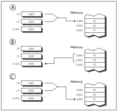
How can we push the segment:offset of the next instruction? Well,
finding the offset of the next instruction by performing a near call to
that instruction is a tried-and-true trick. We can do something similar
here, but in this case we need a far call, since IRET
requires both a segment and an offset. We’ll also branch backward so
that the address pushed on the stack will point to the instruction we
want to continue with. The code works out like this:
jmp short popfskip
popfiret:
iret; branches to the instruction after the
; call, popping the word below the address
; pushed by CALL into the FLAGS register
popfskip:
call far ptr popfiret
;pushes the segment:offset of the next
; instruction on the stack just above
; the flags word, setting things up so
; that IRET will branch to the next
; instruction and pop the flags
; When execution reaches the instruction following this comment,
; the word that was on top of the stack when JMP SHORT POPFSKIP
; was reached has been popped into the FLAGS register, just as
; if a POPF instruction had been executed.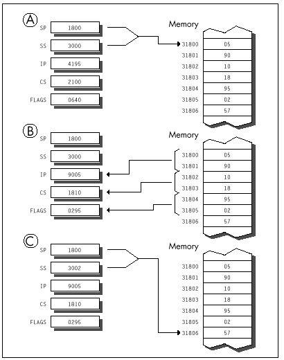
The operation of this code is illustrated in Figure 11.6.
The POPF workaround can best be implemented as a macro;
we can also emulate a far call by pushing CS and performing a near call,
thereby shrinking the workaround code by 1 byte:
EMULATE_POPF macro
local popfskip, popfiret
jmp short popfskip
popfiret:
iret
popfskip:
push cs
call popfiret
endmBy the way, the flags can be popped much more quickly if you’re
willing to alter a register in the process. For example, the following
macro emulates POPF with just one branch, but wipes out
AX:
EMULATE_POPF_TRASH_AX macro
push cs
mov ax,offset $+5
push ax
iret
endmIt’s not a perfect substitute for POPF, since
POPF doesn’t alter any registers, but it’s faster and
shorter than EMULATE_POPF when you can spare the register.
If you’re using 286-specific instructions, you can use which is shorter
still, alters no registers, and branches just once. (Of course, this
version of EMULATE_POPF won’t work on an 8088.)
.286
:
EMULATE_POPFmacro
push cs
push offset $+4
iret
endm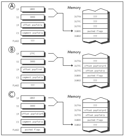
The standard version of EMULATE_POPF is 6 bytes longer
than POPF and much slower, as you’d expect given that it
involves three branches. Anyone in his/her right mind would prefer
POPF to a larger, slower, three-branch macro—given a
choice. In noncode, however, there’s no choice here; the safer—if
slower—approach is the best. (Having people associate your programs with
crashed computers is not a desirable situation, no matter how
unfair the circumstances under which it occurs.)
And now you know the nature of and the workaround for the
POPF bug. Whether you ever need the workaround or not, it’s
a neatly packaged example of the tremendous flexibility of the x86
instruction set.
Chapter 12 – Pushing the 486
It’s Not Just a Bigger 386
So this traveling salesman is walking down a road, and he sees a group of men digging a ditch with their bare hands. “Whoa, there!” he says. “What you guys need is a Model 8088 ditch digger!” And he whips out a trowel and sells it to them.
A few days later, he stops back around. They’re happy with the trowel, but he sells them the latest ditch-digging technology, the Model 80286 spade. That keeps them content until he stops by again with a Model 80386 shovel (a full 32 inches wide, with a narrow point to emulate the trowel), and that holds them until he comes back around with what they really need: a Model 80486 bulldozer.
Having reached the top of the line, the salesman doesn’t pay them a call for a while. When he does, not only are they none too friendly, but they’re digging with the 80386 shovel; the bulldozer is sitting off to one side. “Why on earth are you using that shovel?” the salesman asks. “Why aren’t you digging with the bulldozer?”
“Well, Lord knows we tried,” says the foreman, “but it was all we could do just to lift the damn thing!”
Substitute “processor” for the various digging implements, and you
get an idea of just how different the optimization rules for the 486 are
from what you’re used to. Okay, it’s not quite that bad—but
upon encountering a processor where string instructions are often to be
avoided and memory-to-register MOVs are frequently as fast
as register-to-register MOVs, Dorothy was heard to exclaim
(before she sank out of sight in a swirl of hopelessly mixed metaphors),
“I don’t think we’re in Kansas anymore, Toto.”
Enter the 486
No chip that is a direct, fully compatible descendant of the 8088,
286, and 386 could ever be called a RISC chip, but the 486 certainly
contains RISC elements, and it’s those elements that are most
responsible for making 486 optimization unique. Simple, common
instructions are executed in a single cycle by a RISC-like core
processor, but other instructions are executed pretty much as they were
on the 386, where every instruction takes at least 2 cycles. For
example, MOV AL, [TestChar] takes only 1 cycle on the 486,
assuming both instruction and data are in the cache—3 cycles faster than
the 386—but STOSB takes 5 cycles, 1 cycle slower
than on the 386. The floating-point execution unit inside the 486 is
also much faster than the 387 math coprocessor, largely because, being
in the same silicon as the CPU (the 486 has a math coprocessor built
in), it is more tightly coupled. The results are sometimes startling:
FMUL (floating point multiply) is usually faster on the 486
than IMUL (integer multiply)!
An encyclopedic approach to 486 optimization would take a book all by itself, so in this chapter I’m only going to hit the highlights of 486 optimization, touching on several optimization rules, some documented, some not. You might also want to check out the following sources of 486 information: i486 Microprocessor Programmer’s Reference Manual, from Intel; “8086 Optimization: Aim Down the Middle and Pray,” in the March, 1991 Dr. Dobb’s Journal; and “Peak Performance: On to the 486,” in the November, 1990 Programmer’s Journal.
Rules to Optimize By
In Appendix G of the i486 Microprocessor Programmer’s Reference Manual, Intel lists a number of optimization techniques for the 486. While neither exhaustive (we’ll look at two undocumented optimizations shortly) nor entirely accurate (we’ll correct two of the rules here), Intel’s list is certainly a good starting point. In particular, the list conveys the extent to which 486 optimization differs from optimization for earlier x86 processors. Generally, I’ll be discussing optimization for real mode (it being the most widely used mode at the moment), although many of the rules should apply to protected mode as well.
In other words, for cached code (which time-critical code almost always is), performance is predictable and can be calculated with good precision, and those calculations will apply on any 486. However, “predictable” doesn’t mean “trivial”; the cycle times printed for the various instructions are not the whole story. You must be aware of all the rules, documented and undocumented, that go into calculating actual execution times—and uncovering some of those rules is exactly what this chapter is about.
The Hazards of Indexed Addressing
Rule #1: Avoid indexed addressing (that is, try not to use either two registers or scaled addressing to point to memory).
Intel cautions against using indexing to address memory because there’s a one-cycle penalty for indexed addressing. True enough—but “indexed addressing” might not mean what you expect.
Traditionally, SI and DI are considered the index registers of the
x86 CPUs. That is not the sense in which “indexed addressing” is meant
here, however. In real mode, indexed addressing means that two
registers, rather than one or none, are used to point to memory. (In
this context, the use of one register to address memory is “base
addressing,” no matter what register is used.)
MOV AX, [BX+DI] and MOV CL, [BP+SI+10] perform
indexed addressing; MOV AX,[BX] and
MOV DL, [SI+1] do not.
As an example, you might adhere to this rule by replacing the code
LoopTop:
add ax,[bx+si]
add si,2
dec cx
jnz LoopTopwith this
add si,bx
LoopTop:
add ax,[si]
add si,2
dec cx
jnz LoopTop
sub si,bxwhich calculates the same sum and leaves the registers in the same state as the first example, but avoids indexed addressing.
In protected mode, the definition of indexed addressing is a tad more
complex. The use of two registers to address memory, as in
MOV EAX, [EDX+EDI], still qualifies for the one-cycle
penalty. In addition, the use of 386/486 scaled addressing, as in
MOV [ECX*2],EAX, also constitutes indexed addressing, even
if only one register is used to point to memory.
All this fuss over one cycle! You might well wonder how much
difference one cycle could make. After all, on the 8088, effective
address calculations take a minimum of 5 cycles. On the 486,
however, 1 cycle is a big deal because many instructions, including most
register-only instructions (MOV, ADD,
CMP, and so on) execute in just 1 cycle. In particular,
MOVs to and from memory execute in 1 cycle—if they’re not
hampered by something like indexed addressing, in which case they slow
to half speed (or worse, as we will see shortly).
For example, consider the summing example shown earlier. The version that uses base+index ([BX+SI]) addressing executes in eight cycles per loop. As expected, the version that uses base ([SI]) addressing runs one cycle faster, at seven cycles per loop. However, the loop code executes so fast on the 486 that the single cycle saved by using base addressing makes the whole loop more than 14 percent faster.
In a key loop on the 486, 1 cycle can indeed matter.
Calculate Memory Pointers Ahead of Time
Rule #2: Don’t use a register as a memory pointer during the next two cycles after loading it.
Intel states that if the destination of one instruction is used as the base addressing component of the next instruction, then a one-cycle penalty is imposed. This rule, unlike anything ever before seen in the x86 family, reflects the heavily pipelined nature of the 486. Apparently, the 486 starts each effective address calculation before the start of the instruction that will need it, as shown in Figure 12.1; this effectively makes the address calculation time vanish, because it happens while the preceding instruction executes.
Of course, the 486 can’t perform an effective address calculation for a target instruction ahead of time if one of the address components isn’t known until the instruction starts, and that’s exactly the case when the preceding instruction modifies one of the target instruction’s addressing registers. For example, in the code
MOV BX,OFFSET MemVar
MOV AX,[BX]there’s no way that the 486 can calculate the address referenced by
MOV AX,[BX] until MOV BX,OFFSET MemVar
finishes, so pipelining that calculation ahead of time is not possible.
A good workaround is rearranging your code so that at least one
instruction lies between the loading of the memory pointer and its use.
For example, postdecrementing, as in the following
LoopTop:
add ax,[si]
add si,2
dec cx
jnz LoopTopis faster than preincrementing, as in:
LoopTop:
add si,2
add ax,[SI]
dec cx
jnz LoopTopNow that we understand what Intel means by this rule, let me make a very important comment: My observations indicate that for real-mode code, the documentation understates the extent of the penalty for interrupting the address calculation pipeline by loading a memory pointer just before it’s used.
In 32-bit protected mode, however, the penalty is, in fact, the 1 cycle that Intel .
Considering that MOV normally takes only one cycle
total, that’s quite a loss. For example, the postdecrement loop shown
above is 2 full cycles faster than the preincrement loop, resulting in a
29 percent improvement in the performance of the entire loop. But wait,
there’s more. If a register is loaded 2 cycles (which generally means 2
instructions, but, because some 486 instructions take more than 1
cycle,
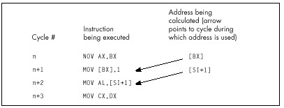
the 2 are not always equivalent) before it’s used to point to memory, 1 cycle is lost. Therefore, whereas this code
mov bx,offset MemVar
mov ax,[bx]
inc dx
dec cx
jnz LoopToploses two cycles from interrupting the address calculation pipeline, this code
mov bx,offset MemVar
inc dx
mov ax,[bx]
dec cx
jnz LoopToploses only one cycle, and this code
mov bx,offset MemVar
inc dx
dec cx
mov ax,[bx]
jnz LoopToploses no cycles at all. Apparently, the 486’s addressing calculation pipeline actually starts 2 cycles ahead, as shown in Figure 12.2. (In truth, my best guess at the moment is that the addressing pipeline really does start only 1 cycle ahead; the additional cycle crops up when the addressing pipeline has to wait for a register to be written into the register file before it can read it out for use in addressing calculations. However, I’m guessing here, and the 2-cycle-ahead model in Figure 12.2 will do just fine for optimization purposes.)
Clearly, there’s considerable optimization potential in careful rearrangement of 486 code.
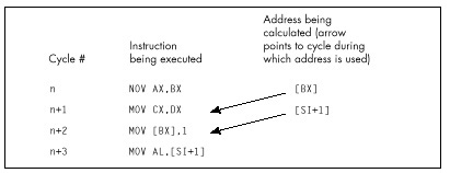
Caveat Programmor
A caution: I’m quite certain that the 2-cycle-ahead addressing pipeline interruption penalty I’ve described exists in the two 486s I’ve tested. However, there’s no guarantee that Intel won’t change this aspect of the 486 in the future, especially given that the documentation indicates otherwise. Perhaps the 2-cycle penalty is the result of a bug in the initial steps of the 486, and will revert to the documented 1-cycle penalty someday; likewise for the undocumented optimizations I’ll describe below. Nonetheless, none of the optimizations I suggest would hurt performance even if the undocumented performance characteristics of the 486 were to vanish, and they certainly will help performance on at least some 486s right now, so I feel they’re well worth using.
There is, of course, no guarantee that I’m entirely correct about the optimizations discussed in this chapter. Without knowing the internals of the 486, all I can do is time code and make inferences from the results; I invite you to deduce your own rules and cross-check them against mine. Also, most likely there are other optimizations that I’m unaware of. If you have further information on these or any other undocumented optimizations, please write and let me know. And, of course, if anyone from Intel is reading this and wants to give us the gospel truth, please do!
Stack Addressing and Address Pipelining
Rule #2A: Rule #2 sometimes, but not always, applies to the stack pointer when it is implicitly used to point to memory.
Intel states that the stack pointer is an implied destination
register for CALL, ENTER, LEAVE,
RET, PUSH, and POP (which alter
(E)SP), and that it is the implied base addressing register for
PUSH, POP, and RET (which use
(E)SP to address memory). Intel then implies that the aforementioned
addressing pipeline penalty is incurred whenever the stack pointer is
used as a destination by one of the first set of instructions and is
then immediately used to address memory by one of the second set. This
raises the specter of unpleasant programming contortions such as
intermixing PUSHes and POPs with other
instructions to avoid interrupting the addressing pipeline. Fortunately,
matters are actually not so grim as Intel’s documentation would
indicate; my tests indicate that the addressing pipeline penalty pops up
only spottily when the stack pointer is involved.
For example, you’d certainly expect a sequence such as
:
pop ax
ret
pop ax
ret
:to exhibit the addressing pipeline interruption phenomenon (SP is
both destination and addressing register for both instructions,
according to Intel), but this code runs in six cycles per
POP/RET pair, matching the official execution times
exactly. Likewise, a sequence like
pop dx
pop cx
pop bx
pop axruns in one cycle per instruction, just as it should.
On the other hand, performing arithmetic directly on SP as an
explicit destination—for example, to deallocate local
variables—and then using PUSH, POP, or
RET, definitely can interrupt the addressing pipeline. For
example
add sp,10h
retloses two cycles because SP is the explicit destination of one instruction and then the implied addressing register for the next, and the sequence
add sp,10h
pop axloses two cycles for the same reason.
I certainly haven’t tried all possible combinations, but the results
so far indicate that the stack pointer incurs the addressing pipeline
penalty only if (E)SP is the explicit destination of one
instruction and is then used by one of the two following instructions to
address memory. So, for instance, SP isn’t the explicit operand of
POP AX-AX is—and no cycles are lost if POP AX
is followed by POP or RET. Happily, then, we
need not worry about the sequence in which we use PUSH and
POP. However, adding to, moving to, or subtracting from the
stack pointer should ideally be done at least two cycles before
PUSH, POP, RET, or any other
instruction that uses the stack pointer to address memory.
Problems with Byte Registers
There are two ways to lose cycles by using byte registers, and neither of them is documented by Intel, so far as I know. Let’s start with the lesser and simpler of the two.
Rule #3: Do not load a byte portion of a register during one instruction, then use that register in its entirety as a source register during the next instruction.
So, for example, it would be a bad idea to do this
mov ah,o
:
mov cx,[MemVar1]
mov al,[MemVar2]
add cx,axbecause AL is loaded by one instruction, then AX is used as the source register for the next instruction. A cycle can be saved simply by rearranging the instructions so that the byte register load isn’t immediately followed by the word register usage, like so:
mov ah,o
:
mov al,[MemVar2]
mov cx,[MemVar1]
add cx,axStrange as it may seem, this rule is neither arbitrary nor nonsensical. Basically, when a byte destination register is part of a word source register for the next instruction, the 486 is unable to directly use the result from the first instruction as the source for the second instruction, because only part of the register required by the second instruction is contained in the first instruction’s result. The full, updated register value must be read from the register file, and that value can’t be read out until the result from the first instruction has been written into the register file, a process that takes an extra cycle. I’m not going to explain this in great detail because it’s not important that you understand why this rule exists (only that it does in fact exist), but it is an interesting window on the way the 486 works.
In case you’re curious, there’s no such penalty for the typical
XLAT sequence like
mov bx,offset MemTable
:
mov al,[si]
xlateven though AL must be converted to a word by XLAT
before it can be added to BX and used to address memory. In fact, none
of the penalties mentioned in this chapter apply to XLAT,
apparently because XLAT is so slow—4 cycles—that it gives
the 486 time to perform addressing calculations during the course of the
instruction.
XLATdoesn’t suffer from the various 486 addressing penalties, the reason for that is basically thatXLATis slow, so there’s still no compelling reason to useXLATon the 486.
In general, penalties for interrupting the 486’s pipeline apply
primarily to the fast core instructions of the 486, most notably
register-only instructions and MOV, although arithmetic and
logical operations that access memory are also often affected. I don’t
know all the performance dependencies, and I don’t plan to; figuring all
of them out would be a big, boring job of little value. Basically, on
the 486 you should concentrate on using those fast core instructions
when performance matters, and all the rules I’ll discuss do indeed apply
to those instructions.
You don’t need to understand every corner of the 486 universe unless you’re a diehard ASMhead who does this stuff for fun. Just learn enough to be able to speed up the key portions of your programs, and spend the rest of your time on a fast design and overall implementation.
More Fun with Byte Registers
Rule #4: Don’t load any byte register exactly 2 cycles before using any register to address memory.
This, the last of this chapter’s rules, is the strangest of the lot. If any byte register is loaded, and then two cycles later any register is used to point to memory, one cycle is lost. So, for example, this code
mov al,bl
mov cx,dx
mov si,[di]takes four rather than the expected three cycles to execute. Note that it is not required that the byte register be part of the register used to address memory; any byte register will do the trick.
Worse still, loading byte registers both one and two cycles before a register is used to address memory costs two cycles, as in
mov bl,al
mov cl,3
mov bx,[si]which takes five rather than three cycles to run. However, there is no penalty if a byte register is loaded one cycle but not two cycles before a register is used to address memory. Therefore,
mov cx,3
mov dl,al
mov si,[bx]runs in the expected three cycles.
In truth, I do not know why this happens. Clearly, it has something to do with interrupting the start of the addressing pipeline, and I have my theories about how this works, but at this point they’re pure speculation. Whatever the reason for this rule, ignorance of it—and of its interaction with the other rules—could lead to considerable performance loss in seemingly air-tight code. For instance, a casual observer would expect the following code to run in 3 cycles:
mov bx,offset MemVar
mov cl,al
mov ax,[bx]A more sophisticated programmer would expect to lose one cycle,
because BX is loaded two cycles before being used to address memory. In
fact, though, this code takes 5 cycles—2 cycles, or 67 percent, longer
than normal. Why? Well, under normal conditions, loading a byte
register—CL in this case—one cycle before using a register to address
memory produces no penalty; loading 2 cycles ahead is the only case that
normally incurs a penalty. However, think of Rule #4 as meaning that
loading a byte register disrupts the memory addressing pipeline as it
starts up. Viewed that way, we can see that
MOV BX,OFFSET MemVar interrupts the addressing pipeline,
forcing it to start again, and then, presumably, MOV CL,AL
interrupts the pipeline again because the pipeline is now on its first
cycle: the one that loading a byte register can affect.
Timing Your Own 486 Code
In case you want to do some 486 performance analysis of your own, let me show you how I arrived at one of the above conclusions; at the same time, I can warn you of the timing hazards of the cache. Listings 12.1 and 12.2 show the code I ran through the Zen timer in order to establish the effects of loading a byte register before using a register to address memory. Listing 12.1 ran in 120 µs on a 33 MHz 486, or 4 cycles per repetition (120 µs/1000 repetitions = 120 ns per repetition; 120 ns per repetition/30 ns per cycle = 4 cycles per repetition); Listing 12.2 ran in 90 µs, or 3 cycles, establishing that loading a byte register costs a cycle only when it’s performed exactly 2 cycles before addressing memory.
LISTING 12.1 LST12-1.ASM
; Measures the effect of loading a byte register 2 cycles before
; using a register to address memory.
mov bp,2 ;run the test code twice to make sure
; it's cached
sub bx,bx
CacheFillLoop:
call ZTimerOn ;start timing
rept 1000
mov dl,cl
nop
mov ax,[bx]
endm
call ZTimerOff ;stop timing
dec bp
jz Done
jmp CacheFillLoop
Done:LISTING 12.2 LST12-2.ASM
; Measures the effect of loading a byte register 1 cycle before
; using a register to address memory.
mov bp,2 ;run the test code twice to make sure
; it's cached
sub bx,bx
CacheFillLoop:
call ZTimerOn ;start timing
rept 1000
nop
mov dl,cl
mov ax,[bx]
endm
call ZTimerOff ;stop timing
dec bp
jz Done
jmp CacheFillLoop
Done:Note that Listings 12.1 and 12.2 each repeat the timing of the code
under test a second time, to make sure that the instructions are in the
cache on the second pass, the one for which results are displayed. Also
note that the code is less than 8K in size, so that it can all fit in
the 486’s 8K internal cache. If I double the REPT value in
Listing 12.2 to 2,000, making the test code larger than 8K, the
execution time more than doubles to 224 µs, or 3.7 cycles per
repetition; the extra seven-tenths of a cycle comes from fetching
non-cached instruction bytes.
The Story Continues
There’s certainly plenty more 486 lore to explore, including the 486’s unique prefetch queue, more optimization rules, branching optimizations, performance implications of the cache, the cost of cache misses for reads, and the implications of cache write-through for writes. Nonetheless, we’ve covered quite a bit of ground in this chapter, and I trust you’ve gotten a feel for the considerable extent to which 486 optimization differs from what you’re used to. Odd as 486 optimization is, though, it’s well worth mastering, for the 486 is, at its best, so staggeringly fast that carefully crafted 486 code can do more than twice as much per cycle as the best 386 code—which makes it perhaps 50 times as fast as optimized code for the original PC.
Sometimes it is hard to believe we’re still in Kansas!
Chapter 13 – Aiming the 486
Pipelines and Other Hazards of the High End
It’s a sad but true fact that 84 percent of American schoolchildren are ignorant of 92 percent of American history. Not my daughter, though. We recently visited historical Revolutionary-War-vintage Fort Ticonderoga, and she’s now 97 percent aware of a key element of our national heritage: that the basic uniform for soldiers in those days was what appears to be underwear, plus a hat so that no one could complain that they were undermining family values. Ha! Just kidding! Actually, what she learned was that in those days, it was pure coincidence if a cannonball actually hit anything it was aimed at, which isn’t surprising considering the lack of rifling, precision parts, and ballistics. The guides at the fort shot off three cannons; the closest they came to the target was about 50 feet, and that was only because the wind helped. I think the idea in early wars was just to put so much lead in the air that some of it was bound to hit something; preferably, but not necessarily, the enemy.
Nowadays, of course, we have automatic weapons that allow a teenager to singlehandedly defeat the entire U.S. Army, not to mention so-called “smart” bombs, which are smart in the sense that they can seek out and empty a taxpayer’s wallet without being detected by radar. There’s an obvious lesson here about progress, which I leave you to deduce for yourselves.
Here’s the same lesson, in another form. Ten years ago, we had a slow processor, the 8088, for which it was devilishly hard to optimize, and for which there was no good optimization documentation available. Now we have a processor, the 486, that’s 50 to 100 times faster than the 8088—and for which there is no good optimization documentation available. Sure, Intel provides a few tidbits on optimization in the back of the i486 Microprocessor Programmer’s Reference Manual, but, as I discussed in Chapter 12, that information is both incomplete and not entirely correct. Besides, most assembly language programmers don’t bother to read Intel’s manuals (which are extremely informative and well done, but only slightly more fun to read than the phone book), and go right on programming the 486 using outdated 8088 optimization techniques, blissfully unaware of a new and heavily mutated generation of cycle-eaters that interact with their code in ways undreamt of even on the 386.
For example, consider how Terje Mathisen doubled the speed of his word-counting program on a 486 simply by shuffling a couple of instructions.
486 Pipeline Optimization
I’ve mentioned Terje Mathisen in my writings before. Terje is an assembly language programmer extraordinaire, and author of the incredibly fast public-domain word-counting program WC (which comes complete with source code; well worth a look, if you want to see what really fast code looks like). Terje’s a regular participant in the ibm.pc/fast.code topic on Bix. In a thread titled “486 Pipeline Optimization, or TANSTATFC (There Ain’t No Such Thing As The Fastest Code),” he detailed the following optimization to WC, perhaps the best example of 486 pipeline optimization I’ve yet seen.
Terje’s inner loop originally looked something like the code in Listing 13.1. (I’ve taken a few liberties for illustrative purposes.) Of course, Terje unrolls this loop a few times (128 times, to be exact). By the way, in Listing 13.1 you’ll notice that Terje counts not only words but also lines, at a rate of three instructions for every two characters!
LISTING 13.1 L13-1.ASM
mov di,[bp+OFFS] ;get the next pair of characters
mov bl,[di] ;get the state value for the pair
add dx,[bx+8000h] ;increment word and line count
; appropriately for the pairListing 13.1 looks as tight as it could be, with just two one-cycle instructions, one two-cycle instruction, and no branches. It is tight, but those three instructions actually take a minimum of 8 cycles to execute, as shown in Figure 13.1. The problem is that DI is loaded just before being used to address memory, and that costs 2 cycles because it interrupts the 486’s internal instruction pipeline. Likewise, BX is loaded just before being used to address memory, costing another two cycles. Thus, this loop takes twice as long as cycle counts would seem to indicate, simply because two registers are loaded immediately before being used, disrupting the 486’s pipeline.
Listing 13.2 shows Terje’s immediate response to these pipelining problems; he simply swapped the instructions that load DI and BL. This one change cut execution time per character pair from eight cycles to five cycles! The load of BL is now separated by one instruction from the use of BX to address memory, so the pipeline penalty is reduced from two cycles to one cycle. The load of DI is also separated by one instruction from the use of DI to address memory (remember, the loop is unrolled, so the last instruction is followed by the first instruction), but because the intervening instruction takes two cycles, there’s no penalty at all.
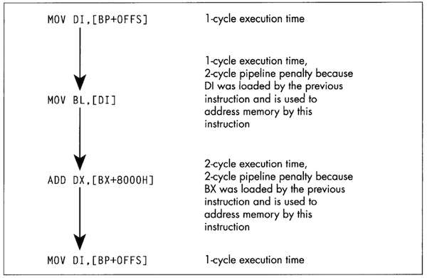
LISTING 13.2 L13-2.ASM
mov bl,[di] ;get the state value for the pair
mov di,[bp+OFFS] ;get the next pair of characters
add dx,[bx+8000h] ;increment word and line count
; appropriately for the pairAt this point, Terje had nearly doubled the performance of this code simply by moving one instruction. (Note that swapping the instructions also made it necessary to preload DI at the start of the loop; Listing 13.2 is not exactly equivalent to Listing 13.1.) I’ll let Terje describe his next optimization in his own words:
“When I looked closely as this, I realized that the two cycles for
the final ADD is just the sum of 1 cycle to load the data
from memory, and 1 cycle to add it to DX, so the code could just as well
have been written as shown in Listing 13.3. The final breakthrough came
when I realized that by initializing AX to zero outside the loop, I
could rearrange it as shown in Listing 13.4 and do the final
ADD DX,AX after the loop. This way there are two
single-cycle instructions between the first and the fourth line,
avoiding all pipeline stalls, for a total throughput of two
cycles/char.”
LISTING 13.3 L13-3.ASM
mov bl,[di] ;get the state value for the pair
mov di,[bp+OFFS] ;get the next pair of characters
mov ax,[bx+8000h] ;increment word and line count
add dx,ax ; appropriately for the pairLISTING 13.4 L13-4.ASM
mov bl,[di] ;get the state value for the pair
mov di,[bp+OFFS] ;get the next pair of characters
add dx,ax ;increment word and line count
; appropriately for the pair
mov ax,[bx+8000h] ;get increments for next timeI’d like to point out two fairly remarkable things. First, the single cycle that Terje saved in Listing 13.4 sped up his entire word-counting engine by 25 percent or more; Listing 13.4 is fully twice as fast as Listing 13.1—all the result of nothing more than shifting an instruction and splitting another into two operations. Second, Terje’s word-counting engine can process more than 16 million characters per second on a 486/33.
Clever 486 optimization can pay off big. QED.
BSWAP: More Useful Than You Might Think
There are only 3 non-system instructions unique to the 486. None is
earthshaking, but they have their uses. Consider BSWAP.
BSWAP does just what its name implies, swapping the bytes
(not bits) of a 32-bit register from one end of the register to the
other, as shown in Figure 13.2. (BSWAP can only work with
32-bit registers; memory locations and 16-bit registers are not valid
operands.) The obvious use of BSWAP is to convert data from
Intel format (least significant byte first in memory, also called
little endian) to Motorola format (most significant byte first
in memory, or big endian), like so:
lodsd
bswap
stosdBSWAP can also be useful for reversing the order of
pixel bits from a bitmap so that they can be rotated 32 bits at a time
with an instruction such as ROR EAX,1. Intel’s byte
ordering for multiword values (least-significant byte first) loads
pixels in the wrong order, so far as word rotation is concerned, but
BSWAP can take care of that.
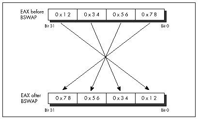
As it turns out, though, BSWAP is also useful in an
unexpected way, having to do with making efficient use of the upper half
of 32-bit registers. As any assembly language programmer knows, the x86
register set is too small; or, to phrase that another way, it sure would
be nice if the register set were bigger. As any 386/486 assembly
language programmer knows, there are many cases in which 16 bits is
plenty. For example, a 16-bit scan-line counter generally does the trick
nicely in a video driver, because there are very few video
devices with more than 65,535 addressable scan lines. Combining these
two observations yields the obvious conclusion that it would be great if
there were some way to use the upper and lower 16 bits of selected 386
registers as separate 16-bit registers, effectively increasing the
available register space.
Unfortunately, the x86 instruction set doesn’t provide any way to work directly with only the upper half of a 32-bit register. The next best solution is to rotate the register to give you access in the lower 16 bits to the half you need at any particular time, with code along the lines of that in Listing 13.5. Having to rotate the 16-bit fields into position certainly isn’t as good as having direct access to the upper half, but surely it’s better than having to get the values out of memory, isn’t it?
LISTING 13.5 L13-5.ASM
mov cx,[initialskip]
shl ecx,16 ;put skip value in upper half of ECX
mov cx,100 ;put loop count in CX
looptop:
:
ror ecx,16 ;make skip value word accessible in CX
add bx,cx ;skip BX ahead
inc cx ;set next skip value
ror ecx,16 ;put loop count in CX
dec cx ;count down loop
jnz looptopNot necessarily. Shifts and rotates are among the worst performing
instructions of the 486, taking 2 to 3 cycles to execute. Thus, it takes
2 cycles to rotate the skip value into CX in Listing 13.5, and 2 more
cycles to rotate it back to the upper half of ECX. I’d say four cycles
is a pretty steep price to pay, especially considering that a
MOV to or from memory takes only one cycle. Basically,
using ROR to access a 16-bit value in the upper half of a
16-bit register is a pretty marginal technique, unless for some reason
you can’t access memory at all (for example, if you’re using BP as a
working register, temporarily making the stack frame inaccessible).
On the 386, ROR was the only way to split a 32-bit
register into two 16-bit registers. On the 486, however,
BSWAP can not only do the job, but can do it better,
because BSWAP executes in just one cycle.
BSWAP has the added benefit of not affecting any flags,
unlike ROR. With BSWAP-based code like that in
Listing 13.6, the upper 16 bits of a register can be accessed with only
2 cycles of overhead and without altering any flags, making the
technique of packing two 16-bit registers into one 32-bit register much
more useful.
LISTING 13.6 L13-6.ASM
mov cx,[initialskip]
bswap ecx ;put skip value in upper half of ECX
mov cx,100 ;put loop count in CX
looptop:
:
bswap ecx ;make skip value word accessible in CX
add bx,cx ;skip BX ahead
inc cx ;set next skip value
bswap ecx ;put loop count in CX
dec cx ;count down loop
jnz looptopPushing and Popping Memory
Pushing or popping a memory location, as in
PUSH WORD PTR [BX] or POP [MemVar], is a
compact, easy way to get a value onto or off of the stack, especially
when pushing parameters for calling a C-compatible function. However, on
a 486, these are unattractive instructions from a performance
perspective. Pushing a memory location takes four cycles; by contrast,
loading a memory location into a register takes only one cycle, and
pushing a register takes just 1 more cycle, for a total of two cycles.
Therefore,
mov ax,[bx]
push axis twice as fast as
push word ptr [bx]and the only cost is that the previous contents of AX are destroyed.
Likewise, popping a memory location takes six cycles, but popping a register and writing it to memory takes only two cycles combined. The i486 Microprocessor Programmer’s Reference Manual lists a 4-cycle execution time for popping a register, but pay that no mind; popping a register takes only 1 cycle.
Why is it that such a convenient operation as pushing or popping
memory is so slow? The rule on the 486 is that simple operations, which
can be executed in a single cycle by the 486’s RISC core, are fast;
whereas complex operations, which must be carried out in microcode just
as they were on the 386, are almost all relatively slow. Slow, complex
operations include all the string instructions except
REP MOVS, as well as XLAT, LOOP,
and, of course, PUSH *mem* and POP *mem*.
MOV,ADD,SUB,CMP,ADC,SBB,XOR,AND,OR,TEST,LEA, andPUSH regandPOP reg. These instructions have an added benefit in that it’s often possible to rearrange them for maximum pipeline efficiency, as is the case with Terje’s optimization described earlier in this chapter.
Optimal 1-Bit Shifts and Rotates
On a 486, the n-bit forms of the shift and rotate instructions—as in
ROR AX,2 and SHL BX,9—are 2-cycle
instructions, but the 1-bit forms—as in ROR AX,1 and
SHL BX,1-are 3-cycle instructions. Go figure.
Assemblers default to the 1-bit instruction for 1-bit shifts and
rotates. That’s not unreasonable since the 1-bit form is a byte shorter
and is just as fast as the n-bit forms on a 386 and faster on a 286, and
the n-bit form doesn’t even exist on an 8088. In a really critical loop,
however, it might be worth hand-assembling the n-bit form of a
single-bit shift or rotate in order to save that cycle. The easiest way
to do this is to assemble a 2-bit form of the desired instruction, as in
SHL AX,2, then look at the hex codes that the assembler
generates and use DB to insert them in your program code,
with the value two replaced with the value one. For example, you could
determine that SHL AX,2 assembles to the bytes 0C1H 0E0H
002H, either by looking at the disassembly in a debugger or by having
the assembler generate a listing file. You could then insert the n-bit
version of SHL AX,1 in your code as follows:
mov ax,1
db 0c1h, 0e0h, 001h
mov dx,axAt the end of this sequence, DX will contain 2, and the fast n-bit
version of SHL AX,1 will have executed. If you use this
approach, I’d recommend using a macro, rather than sticking DBs in the
middle of your code.
Again, this technique is advantageous only on a 486. It also
doesn’t apply to RCL and RCR, where you
definitely want to use the 1-bit versions whenever you can, because the
n-bit versions are horrendously slow. But if you’re optimizing for the
486, these tidbits can save a few critical cycles—and Lord knows that if
you’re optimizing for the 486—that is, if you need even more performance
than you get from unoptimized code on a 486—you almost certainly need
all the speed you can get.
32-Bit Addressing Modes
The 386 and 486 both support 32-bit addressing modes, in which any register may serve as the base memory addressing register, and almost any register may serve as the potentially scaled index register. For example,
mov al,BaseTable[ecx+edx*4]uses a perfectly valid 32-bit address, with the byte accessed being
the one at the offset in DS pointed to by the sum of EDX times 4 plus
the offset of BaseTable plus ECX. This is a very powerful
memory addressing scheme, far superior to 8088-style 16-bit addressing,
but it’s not without its quirks and costs, so let’s take a quick look at
32-bit addressing. (By the way, 32-bit addressing is not limited to
protected mode; 32-bit instructions may be used in real mode, although
each instruction that uses 32-bit addressing must have an address-size
prefix byte, and the presence of a prefix byte costs a cycle on a
486.)
Any register may serve as the base register component of an address. Any register except ESP may also serve as the index register, which can be scaled by 1, 2, 4, or 8. (Scaling is very handy for performing lookups in arrays and tables.) The same register may serve as both base and index register, except for ESP, which can only be the base. Incidentally, it makes sense that ESP can’t be scaled; ESP presumably always points to a valid stack, and I can’t think of any reason you’d want to use the stack pointer times 2, 4, or 8 in an address. ESP is, by its nature, a base rather than index pointer.
That’s all there is to the functionality of 32-bit addressing; it’s
very simple, much simpler than 16-bit addressing, with its sharply
limited memory addressing register combinations. The costs of 32-bit
addressing are a bit more subtle. The only performance cost (apart from
the aforementioned 1-cycle penalty for using 32-bit addressing in real
mode) is a 1-cycle penalty imposed for using an index register. In this
context, you use an index register when you use a register that’s
scaled, or when you use the sum of two registers to point to memory.
MOV BL,[EBX*2] uses an index register and takes an extra
cycle, as does MOV CL,[EAX+EDX]; MOV CL,[EAX+100H] is not
indexed, however.
The other cost of 32-bit addressing is in instruction size. Old-style
16-bit addressing usually (except in a few special cases) uses one extra
byte, which Intel calls the Mod-R/M byte, which is placed immediately
after each instruction’s opcode to describe the memory addressing mode,
plus 1 or 2 optional bytes of addressing displacement—that is, a
constant value to add into the address. In many cases, 32-bit addressing
continues to use the Mod-R/M byte, albeit with a different
interpretation; in these cases, 32-bit addressing is no larger than
16-bit addressing, except when a 32-bit displacement is involved. For
example, MOV AL, [EBX] is a 2-byte instruction;
MOV AL, [EBX+10H] is a 3-byte instruction; and
MOV AL, [EBX+10000H] is a 6-byte instruction.
However, because 32-bit addressing supports many more addressing combinations than 16-bit addressing, the Mod-R/M byte can’t describe all the combinations. Therefore, whenever an index register (as described above) is involved, a second byte, the SIB byte, follows the Mod-R/M byte to provide additional address information. Consequently, whenever you use a scaled memory addressing register or use the sum of two registers to point to memory, you automatically add 1 cycle and 1 byte to that instruction. This is not to say that you shouldn’t use index registers when they’re needed, but if you find yourself using them inside key loops, you should see if it’s possible to move the index calculation outside the loop as, for example, in a loop like this:
LoopTop:
add ax,DataTable[ebx*2]
inc ebx
dec cx
jnz LoopTopYou could change this to the following for greater performance:
add ebx,ebx ;ebx*2
LoopTop:
add ax,DataTable[ebx]
add ebxX,2
dec cx
jnz LoopTop
shr ebx,1 ;ebx*2/2I’ll end this chapter with two more quirks of 32-bit addressing. First, as with 16-bit addressing, addressing that uses EBP as a base register both accesses the SS segment by default and always has a displacement of at least 1 byte. This reflects the common use of EBP to address a stack frame, but is worth keeping in mind if you should happen to use EBP to address non-stack memory.
Lastly, as I mentioned, ESP cannot be scaled. In fact, ESP cannot be an index register; it must be a base register. Ironically, however, ESP is the one register that cannot be used to address memory without the presence of an SIB byte, even if it’s used without an index register. This is an outcome of the way in which the SIB byte extends the capabilities of the Mod-R/M byte, and there’s nothing to be done about it, but it’s at least worth noting that ESP-based, non-indexed addressing makes for instructions that are a byte larger than other non-indexed addressing (but not any slower; there’s no 1-cycle penalty for using ESP as a base register) on the 486.
Chapter 14 – Boyer-Moore String Searching
Optimizing a Pretty Optimum Search Algorithm
When you seem to be stumped, stop for a minute and think. All the information you need may be right in front of your nose if you just look at things a little differently. Here’s a case in point:
When I was in college, I used to stay around campus for the summer. Oh, I’d take a course or two, but mostly it was an excuse to hang out and have fun. In that spirit, my girlfriend, Adrian (not my future wife, partly for reasons that will soon become apparent), bussed in to spend a week, sharing a less-than-elegant $150 per month apartment with me and, by necessity, my roommate.
Our apartment was pretty much standard issue for two male college students; maybe even a cut above. The dishes were usually washed, there was generally food in the refrigerator, and nothing larger than a small dog had taken up permanent residence in the bathroom. However, there was one sticking point (literally): the kitchen floor. This floor—standard tile, with a nice pattern of black lines on an off-white background (or so we thought)—had never been cleaned. By which I mean that I know for a certainty that we had never cleaned it, but I suspect that it had in fact not been cleaned since the Late Jurassic, or possibly earlier. Our feet tended to stick to it; had the apartment suddenly turned upside-down, I think we’d all have been hanging from the ceiling.
One day, my roommate and I returned from a pick-up basketball game. Adrian, having been left to her own devices for a couple of hours, had apparently kept herself busy. “Notice anything?” she asked, with an edge to her voice that suggested we had damned well better.
“Uh, you cooked dinner?” I guessed. “Washed the dishes? Had your hair done?” My roommate was equally without a clue.
She stamped her foot (really; the only time I’ve ever seen it happen), and said, “No, you jerks! The kitchen floor! Look at the floor! I cleaned it!”
The floor really did look amazing. It was actually all white; the black lines had been grooves filled with dirt. We assured her that it looked terrific, it just wasn’t that obvious until you knew to look for it; anyone would tell you that it wasn’t the kind of thing that jumped out at you, but it really was great, no kidding. We had almost smoothed things over, when a friend walked in, looked around with a start, and said, “Hey! Did you guys put in a new floor?”
As I said, sometimes everything you need to know is right in front of your nose. Which brings us to Boyer-Moore string searching.
String Searching Refresher
I’ve discussed string searching earlier in this book, in Chapters 5
and 9. You may want to refer back to these chapters for some background
on string searching in general. I’m also going to use some of the code
from that chapter as part of this chapter’s test suite. For further
information, you may want to refer to the discussion of string searching
in the excellent Algorithms in C, by Robert Sedgewick
(Addison-Wesley), which served as the primary reference for this
chapter. (If you look at Sedgewick, be aware that in the Boyer-Moore
listing on page 288, there is a mistake: “j > 0” in the
for loop should be “j >= 0,” unless I’m missing
something.)
String searching is the simple matter of finding the first occurrence
of a particular sequence of bytes (the pattern) within another sequence
of bytes (the buffer). The obvious, brute-force approach is to try every
possible match location, starting at the beginning of the buffer and
advancing one position after each mismatch, until either a match is
found or the buffer is exhausted. There’s even a nifty string
instruction, REPZ CMPS, that’s perfect for comparing the
pattern to the contents of the buffer at each location. What could be
simpler?
We have some important information that we’re not yet using, though.
Typically, the buffer will contain a wide variety of bytes. Let’s assume
that the buffer contains text, in which case there will be dozens of
different characters; and although the distribution of characters won’t
usually be even, neither will any one character constitute half the
buffer, or anything close. A reasonable conclusion is that the first
character of the pattern will rarely match the first character of the
buffer location currently being checked. This allows us to use the
speedy REPNZ SCASB to whiz through the buffer, eliminating
most potential match locations with single repetitions of
SCASB. Only when that first character does (infrequently)
match must we drop back to the slower REPZ CMPS
approach.
It’s important to understand that we’re assuming that the buffer is typical text. That’s what I meant at the outset, when I said that the information you need may be under your nose.
If the buffer contains the letter ‘A’ repeated 1,000 times, followed
by the letter ‘B,’ then the REPNZ SCASB/REPZ CMPS approach
will be much slower than the brute-force REPZ CMPS approach
when searching for the pattern “AB,” because REPNZ SCASB
would match at every buffer location. You could construct a horrendous
worst-case scenario for almost any good optimization; the key is
understanding the usual conditions under which your code will work.
As discussed in Chapter 9, we also know that certain characters have
lower probabilities of matching than others. In a normal buffer, ‘T’
will match far more often than ‘X.’ Therefore, if we use
REPNZ SCASB to scan for the least common letter in the
search string, rather than the first letter, we’ll greatly decrease the
number of times we have to drop back to REPZ CMPS, and the
search time will become very close to the time it takes
REPNZ SCASB to go from the start of the buffer to the match
location. If the distance to the first match is N bytes, the
least-common REPNZ SCASB approach will take about as long
as N repetitions of REPNZ SCASB.
At this point, we’re pretty much searching at the speed of
REPNZ SCASB. On the x86, there simply is no faster way to
test each character in turn. In order to get any faster, we’d have to
check fewer characters—but we can’t do that and still be sure of finding
all matches. Can we?
Actually, yes, we can.
The Boyer-Moore Algorithm
All our a priori knowledge of string searching is stated above, but there’s another sort of knowledge—knowledge that’s generated dynamically. As we search through the buffer, we acquire information each time we check for a match. One sort of information that we acquire is based on partial matches; we can often skip ahead after partial matches because (take a deep breath!) by partially matching, we have already implicitly done a comparison of the partially matched buffer characters with all possible pattern start locations that overlap those partially-matched bytes.
If that makes your head hurt, it should—and don’t worry. This line of thinking, which is the basis of the Knuth-Morris-Pratt algorithm and half the basis of the Boyer-Moore algorithm, is what gives Boyer-Moore its reputation for inscrutability. That reputation is well deserved for this aspect (which I will not discuss further in this book), but there’s another part of Boyer-Moore that’s easily understood, easily implemented, and highly effective.
Consider this: We’re searching for the pattern “ABC,” beginning the search at the start (offset 0) of a buffer containing “ABZABC.” We match on ‘A,’ we match on ‘B,’ and we mismatch on ‘C’; the buffer contains a ‘Z’ in this position. What have we learned? Why, we’ve learned not only that the pattern doesn’t match the buffer starting at offset 0, but also that it can’t possibly match starting at offset 1 or offset 2, either! After all, there’s a ‘Z’ in the buffer at offset 2; since the pattern doesn’t contain a single ‘Z,’ there’s no way that the pattern can match starting at any location from which it would span the ‘Z’ at offset 2. We can just skip straight from offset 0 to offset 3 and continue, saving ourselves two comparisons.
Unfortunately, this approach only pays off big when a near-complete
partial match is found; if the comparison fails on the first pattern
character, as often happens, we can only skip ahead 1 byte, as usual.
Look at it differently, though: What if we compare the pattern starting
with the last (rightmost) byte, rather than the first (leftmost) byte?
In other words, what if we compare from high memory toward low, in the
direction in which string instructions go after the STD
instruction? After all, we’re comparing one set of bytes (the pattern)
to another set of bytes (a portion of the buffer); it doesn’t matter in
the least in what order we compare them, so long as all the bytes in one
set are compared to the corresponding bytes in the other set.
We learn nothing new from a mismatch on the leftmost character,
except that the pattern can’t match starting at that location. A
mismatch on the rightmost character, however, tells us about the
possibilities of the pattern matching starting at every buffer location
from which the pattern spans the mismatch location. If the mismatched
character in the buffer doesn’t appear in the pattern, then we’ve just
eliminated not one potential match, but as many potential matches as
there are characters in the pattern; that’s how many locations there are
in the buffer that might have matched, but have just been shown
not to, because they overlap the mismatched character that doesn’t
belong in the pattern. In this case, we can skip ahead by the full
pattern length in the buffer! This is how we can outperform even
REPNZ SCASB; REPNZ SCASB has to check every byte in the
buffer, but Boyer-Moore doesn’t.
Figure 14.1 illustrates the operation of a Boyer-Moore search when the rightcharacter of the search pattern (which is the first character that’s compared at each location because we’re comparing backwards) mismatches with a buffer character that appears nowhere in the pattern. Figure 14.2 illustrates the operation of a partial match when the mismatch occurs with a character that’s not a pattern member. In this case, we can only skip ahead past the mismatch location, resulting in an advance of fewer bytes than the pattern length, and potentially as little as the same single byte distance by which the standard search approach advances.
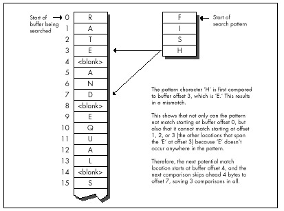
What if the mismatch occurs with a buffer character that does occur in the pattern? Then we can’t skip past the mismatch location, but we can skip to whatever location aligns the rightmost occurrence of that character in the pattern with the mismatch location, as shown in Figure 14.3.
Basically, we exercise our right as members of a free society to compare strings in whichever direction we choose, and we choose to do so right to left, rather than the more intuitive left to right. Whenever we find a mismatch, we see what we can learn from the buffer character that failed to match the pattern. Imagine that we move the pattern to the right across the mismatch location until we find a start location that the mismatch does not eliminate as a possible match for the pattern. If the mismatch character doesn’t appear in the pattern, the pattern can move clear past the mismatch location. Otherwise, the pattern moves until a matching pattern byte lies atop the mismatch. That’s all there is to it!
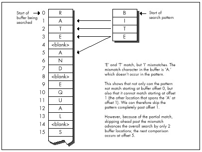
Boyer-Moore: The Good and the Bad
The worst case for this version of Boyer-Moore is that the pattern mismatches on the leftmost character—the last character compared—every time. Again, not very likely, but it is true that this version of Boyer-Moore performs better as there are fewer and shorter partial matches; ideally, the rightmost character would never match until the full match location was reached. Longer patterns, which make for longer skips, help Boyer-Moore, as does a long distance to the match location, which helps diffuse the overhead of building the table of distances to skip ahead on all the possible mismatch values.
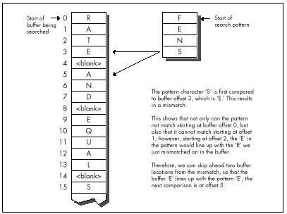
The best case for Boyer-Moore is good indeed: About N/M comparisons are required, where N is the buffer length and M is the pattern length. This reflects the ability of Boyer-Moore to skip ahead by a full pattern length on a complete mismatch.
How fast is Boyer-Moore? Listing 14.1 is a C implementation
of Boyer-Moore searching; Listing 14.2 is a test-bed program that
searches up to the first 32K of a file for a pattern. Table 14.1 (all
times measured with Turbo Profiler on a 20 MHz cached 386, searching a
modified version of the text of this chapter) shows that this
implementation is generally much slower than REPNZ SCASB,
although it does come close when searching for long patterns. Listing
14.1 is designed primarily to make later assembly implemenmore
comprehensible, rather than faster; Sedge’s implementation uses arrays
rather than pointers, is a great deal more compact and very clever, and
may be somewhat faster. Regardless, the far superior performance of
REPNZ SCASB clearly indicates that assembly language is in
order at this point.
| “g;” | “Yogi” | “igoY” | “Adrian” | “Conclusion” | “You don’t know what you know” | |
|---|---|---|---|---|---|---|
| Searching approach | (16K) | (16K) | (16K) | (<1K) | (16K) | (16K) |
| REPNZ SCASB on first char a (Listing 9.1) | 8.2 | 7.5 | 9.7 | 0.4 | 7.4 | 8.1 |
| REPNZ SCASB on least common char (Listing 9.2) | 7.6 | 7.5 | 7.5 | 0.5 | 7.5 | 7.5 |
| Boyer-Moore in C (Listing 14.1) | 71.0 | 38.4 | 37.7 | 1.8 | 18.2 | 9.2 |
| Standard Boyer-Moore in ASM (code not shown) | 38.5 | 21.0 | 20.5 | 0.8 | 9.4 | 4.8 |
| Quick handling of first mismatch Boyer-Moore in ASM (Listing 14.3) | 14.1 | 8.9 | 7.7 | 0.4 | 4.0 | 2.0 |
| <=255 pattern length + sentinelBoyer-Moore in ASM (Listing 14.4) | 8.1 | 5.2 | 4.6 | 0.3 | 2.6 | 1.2 |
Search pattern (approximate distance searched before match is shown
in parentheses).
Times are in milliseconds; shorter is better.
The entry “Standard Boyer-Moore in ASM” in Table 14.1 refers to
straight-forward hand optimization of Listing 14.1, code that is not
included in this chapter for the perfectly good reason that it is slower
in most cases than REPNZ SCASB. I say this casually now,
but not so yesterday, when I had all but concluded that Boyer-Moore was
simply inferior on the x86, due to two architectural quirks: the string
instructions and slow branch. I had even coined a neat phrase for it:
Architecture is destiny. Has a nice ring, doesn’t it?
LISTING 14.1 L14-1.C
/* Searches a buffer for a specified pattern. In case of a mismatch,
uses the value of the mismatched byte to skip across as many
potential match locations as possible (partial Boyer-Moore).
Returns start offset of first match searching forward, or NULL if
no match is found.
Tested with Borland C++ in C mode and the small model. */
#include <stdio.h>
unsigned char * FindString(unsigned char * BufferPtr,
unsigned int BufferLength, unsigned char * PatternPtr,
unsigned int PatternLength)
{
unsigned char * WorkingPatternPtr, * WorkingBufferPtr;
unsigned int CompCount, SkipTable[256], Skip, DistanceMatched;
int i;
/* Reject if the buffer is too small */
if (BufferLength < PatternLength) return(NULL);
/* Return an instant match if the pattern is 0-length */
if (PatternLength == 0) return(BufferPtr);
/* Create the table of distances by which to skip ahead on
mismatches for every possible byte value */
/* Initialize all skips to the pattern length; this is the skip
distance for bytes that don't appear in the pattern */
for (i = 0; i < 256; i++) SkipTable[i] = PatternLength;
/*Set the skip values for the bytes that do appear in the pattern
to the distance from the byte location to the end of the
pattern. When there are multiple instances of the same byte,
the rightmost instance's skip value is used. Note that the
rightmost byte of the pattern isn't entered in the skip table;
if we get that value for a mismatch, we know for sure that the
right end of the pattern has already passed the mismatch
location, so this is not a relevant byte for skipping purposes */
for (i = 0; i < (PatternLength - 1); i++)
SkipTable[PatternPtr[i]] = PatternLength - i - 1;
/* Point to rightmost byte of the pattern */
PatternPtr += PatternLength - 1;
/* Point to last (rightmost) byte of the first potential pattern
match location in the buffer */
BufferPtr += PatternLength - 1;
/* Count of number of potential pattern match locations in
buffer */
BufferLength -= PatternLength - 1;
/* Search the buffer */
while (1) {
/* See if we have a match at this buffer location */
WorkingPatternPtr = PatternPtr;
WorkingBufferPtr = BufferPtr;
CompCount = PatternLength;
/* Compare the pattern and the buffer location, searching from
high memory toward low (right to left) */
while (*WorkingPatternPtr— == *WorkingBufferPtr—) {
/* If we've matched the entire pattern, it's a match */
if (-CompCount == 0)
/* Return a pointer to the start of the match location */
return(BufferPtr - PatternLength + 1);
}
/* It's a mismatch; let's see what we can learn from it */
WorkingBufferPtr++; /* point back to the mismatch location */
/* # of bytes that did match */
DistanceMatched = BufferPtr - WorkingBufferPtr;
/*If, based on the mismatch character, we can't even skip ahead
as far as where we started this particular comparison, then
just advance by 1 to the next potential match; otherwise,
skip ahead from the mismatch location by the skip distance
for the mismatch character */
if (SkipTable[*WorkingBufferPtr] <= DistanceMatched)
Skip = 1; /* skip doesn't do any good, advance by 1 */
else
/* Use skip value, accounting for distance covered by the
partial match */
Skip = SkipTable[*WorkingBufferPtr] - DistanceMatched;
/* If skipping ahead would exhaust the buffer, we're done
without a match */
if (Skip >= BufferLength) return(NULL);
/* Skip ahead and perform the next comparison */
BufferLength -= Skip;
BufferPtr += Skip;
}
}LISTING 14.2 L14-2.C
/* Program to exercise buffer-search routines in Listings 14.1 & 14.3.
(Must be modified to put copy of pattern as sentinel at end of the
search buffer in order to be used with Listing 14.4.) */
#include <stdio.h>
#include <string.h>
#include <fcntl.h>
#define DISPLAY_LENGTH 40
#define BUFFER_SIZE 0x8000
extern unsigned char * FindString(unsigned char *, unsigned int,
unsigned char *, unsigned int);
void main(void);
void main() {
unsigned char TempBuffer[DISPLAY_LENGTH+1];
unsigned char Filename[150], Pattern[150], *MatchPtr, *TestBuffer;
int Handle;
unsigned int WorkingLength;
printf("File to search:");
gets(Filename);
printf("Pattern for which to search:");
gets(Pattern);
if ( (Handle = open(Filename, O_RDONLY | O_BINARY)) == -1 ) {
printf("Can't open file: %s\n", Filename); exit(1);
}
/* Get memory in which to buffer the data */
if ( (TestBuffer=(unsigned char *)malloc(BUFFER_SIZE+1)) == NULL) {
printf("Can't get enough memory\n"); exit(1);
}
/* Process a BUFFER_SIZE chunk */
if ( (int)(WorkingLength =
read(Handle, TestBuffer, BUFFER_SIZE)) == -1 ) {
printf("Error reading file %s\n", Filename); exit(1);
}
TestBuffer[WorkingLength] = 0; /* 0-terminate buffer for printf */
/* Search for the pattern and report the results */
if ((MatchPtr = FindString(TestBuffer, WorkingLength, Pattern,
(unsigned int) strlen(Pattern))) == NULL) {
/* Pattern wasn't found */
printf("\"%s\" not found\n", Pattern);
} else {
/* Pattern was found. Zero-terminate TempBuffer; strncpy
won't do it if DISPLAY_LENGTH characters are copied */
TempBuffer[DISPLAY_LENGTH] = 0;
printf("\"%s\" found. Next %d characters at match:\n\"%s\"\n",
Pattern, DISPLAY_LENGTH,
strncpy(TempBuffer, MatchPtr, DISPLAY_LENGTH));
}
exit(0);
}Well, architecture carries a lot of weight, but it sure as heck isn’t
destiny. I had simply fallen into the trap of figuring that the
algorithm was so clever that I didn’t have to do any thinking myself.
The path leading to REPNZ SCASB from the original
brute-force approach of REPZ CMPSB at every location had
been based on my observation that the first character comparison at each
buffer location usually fails. Why not apply the same concept to
Boyer-Moore? Listing 14.3 is just like the standard
implementation—except that it’s optimized to handle a first-comparison
mismatch as quickly as possible in the loop at
QuickSearchLoop, much as REPNZ SCASB optimizes
first-comparison mismatches for the brute-force approach. The results in
Table 14.1 speak for themselves; Listing 14.3 is more than twice as fast
as what I assure you was already a nice, tight assembly implementation
(and unrolling QuickSearchLoop could boost performance by
up to 10 percent more). Listing 14.3 is also four times faster
than REPNZ SCASB in one case.
LISTING 14.3 L14-3.ASM
; Searches a buffer for a specified pattern. In case of a mismatch,
; uses the value of the mismatched byte to skip across as many
; potential match locations as possible (partial Boyer-Moore).
; Returns start offset of first match searching forward, or NULL if
; no match is found.
; Tested with TASM.
; C near-callable as:
; unsigned char * FindString(unsigned char * BufferPtr,
; unsigned int BufferLength, unsigned char * PatternPtr,
; unsigned int PatternLength);
parms struc
dw 2 dup(?) ;pushed BP & return address
BufferPtr dw ? ;pointer to buffer to be searched
BufferLength dw ? ;# of bytes in buffer to be searched
PatternPtr dw ? ;pointer to pattern for which to search
PatternLength dw ? ;length of pattern for which to search
parms ends
.model small
.code
public _FindString
_FindString proc near
cld
push bp ;preserve caller's stack frame
mov bp,sp ;point to our stack frame
push si ;preserve caller's register variables
push di
sub sp,256*2 ;allocate space for SkipTable
; Create the table of distances by which to skip ahead on mismatches
; for every possible byte value. First, initialize all skips to the
; pattern length; this is the skip distance for bytes that don't
; appear in the pattern.
mov ax,[bp+PatternLength]
and ax,ax ;return an instant match if the pattern is
jz InstantMatch ;0-length
mov di,ds
mov es,di ;ES=DS=SS
mov di,sp ;point to SkipBuffer
mov cx,256
rep stosw
dec ax ;from now on, we only need
mov [bp+PatternLength],ax ; PatternLength - 1
; Point to last (rightmost) byte of first potential pattern match
; location in buffer.
add [bp+BufferPtr],ax
; Reject if buffer is too small, and set the count of the number of
; potential pattern match locations in the buffer.
sub [bp+BufferLength],ax
jbe NoMatch
; Set the skip values for the bytes that do appear in the pattern to
; the distance from the byte location to the end of the pattern.
; When there are multiple instances of the same byte, the rightmost
; instance's skip value is used. Note that the rightmost byte of the
; pattern isn't entered in the skip table; if we get that value for
; a mismatch, we know for sure that the right end of the pattern has
; already passed the mismatch location, so this is not a relevant byte
; for skipping purposes.
mov si,[bp+PatternPtr] ;point to start of pattern
and ax,ax ;are there any skips to set?
jz SetSkipDone ;no
mov di,sp ;point to SkipBuffer
SetSkipLoop:
sub bx,bx ;prepare for word addressing off byte value
mov bl,[si] ;get the next pattern byte
inc si ;advance the pattern pointer
shl bx,1 ;prepare for word lookup
mov [di+bx],ax ;set the skip value when this byte value is
; the mismatch value in the buffer
dec ax
jnz SetSkipLoop
SetSkipDone:
mov dl,[si] ;DL=rightmost pattern byte from now on
dec si ;point to next-to-rightmost byte of pattern
mov [bp+PatternPtr],si ; from now on
; Search the buffer.
std ;for backward REPZ CMPSB
mov di,[bp+BufferPtr] ;point to first search location
mov cx,[bp+BufferLength] ;# of match locations to check
SearchLoop:
mov si,sp ;point SI to SkipTable
; Skip through until there's a match for the rightmost pattern byte.
QuickSearchLoop:
mov bl,[di] ;rightmost buffer byte at this location
cmp dl,bl ;does it match the rightmost pattern byte?
jz FullCompare ;yes, so keep going
sub bh,bh ;convert to a word
add bx,bx ;prepare for look-up in SkipTable
mov ax,[si+bx] ;get skip value from skip table for this
; mismatch value
add di,ax ;BufferPtr += Skip;
sub cx,ax ;BufferLength -= Skip;
ja QuickSearchLoop ;continue if any buffer left
jmp short NoMatch
; Return a pointer to the start of the buffer (for 0-length pattern).
align 2
InstantMatch:
mov ax,[bp+BufferPtr]
jmp short Done
; Compare the pattern and the buffer location, searching from high
; memory toward low (right to left).
align 2
FullCompare:
mov [bp+BufferPtr],di ;save the current state of
mov [bp+BufferLength],cx ; the search
mov cx,[bp+PatternLength] ;# of bytes yet to compare
jcxz Match ;done if only one character
mov si,[bp+PatternPtr] ;point to next-to-rightmost bytes
dec di ; of buffer location and pattern
repz cmpsb ;compare the rest of the pattern
jz Match ;that's it; we've found a match
; It's a mismatch; let's see what we can learn from it.
inc di ;compensate for 1-byte overrun of REPZ CMPSB;
; point to mismatch location in buffer
; # of bytes that did match.
mov si,[bp+BufferPtr]
sub si,di
; If, based on the mismatch character, we can't even skip ahead as far
; as where we started this particular comparison, then just advance by
; 1 to the next potential match; otherwise, skip ahead from this
; comparison location by the skip distance for the mismatch character,
; less the distance covered by the partial match.
sub bx,bx ;prepare for word addressing off byte value
mov bl,[di] ;get the value of the mismatch byte in buffer
add bx,bx ;prepare for word look-up
add bx,sp ;SP points to SkipTable
mov cx,[bx] ;get the skip value for this mismatch
mov ax,1 ;assume we'll just advance to the next
; potential match location
sub cx,si ;is the skip far enough to be worth taking?
jna MoveAhead ;no, go with the default advance of 1
mov ax,cx ;yes; this is the distance to skip ahead from
; the last potential match location checked
MoveAhead:
; Skip ahead and perform the next comparison, if there's any buffer
; left to check.
mov di,[bp+BufferPtr]
add di,ax ;BufferPtr += Skip;
mov cx,[bp+BufferLength]
sub cx,ax ;BufferLength -= Skip;
ja SearchLoop ;continue if any buffer left
; Return a NULL pointer for no match.
align 2
NoMatch:
sub ax,ax
jmp short Done
; Return start of match in buffer (BufferPtr - (PatternLength - 1)).
align 2
Match:
mov ax,[bp+BufferPtr]
sub ax,[bp+PatternLength]
Done:
cld ;restore default direction flag
add sp,256*2 ;deallocate space for SkipTable
pop di ;restore caller's register variables
pop si
pop bp ;restore caller's stack frame
ret
_FindString endp
endTable 14.1 represents a limited and decidedly unscientific comparison
of searching techniques. Nonetheless, the overall trend is clear: For
all but the shortest patterns, well-implemented Boyer-Moore is generally
as good as or better than—sometimes much better
than—brute-force searching. (For short patterns, you might want to use
REPNZ SCASB, thereby getting the best of both worlds.)
Know your data and use your smarts. Don’t stop thinking just because you’re implementing a big-name algorithm; you know more than it does.
Further Optimization of Boyer-Moore
We can do substantially better yet than Listing 14.3 if we’re willing
to accept tighter limits on the data. Limiting the length of the
searched-for pattern to a maximum of 255 bytes allows us to use the
XLAT instruction and generally tighten the critical loop.
(Be aware, however, that XLAT is a relatively expensive
instruction on the 486 and Pentium.) Putting a copy of the searched-for
string at the end of the search buffer as a sentinel, so that the search
never fails, frees us from counting down the buffer length, and makes it
easy to unroll the critical loop. Listing 14.4, which implements these
optimizations, is about 60 percent faster than Listing 14.3.
LISTING 14.4 L14-4.ASM
; Searches a buffer for a specified pattern. In case of a mismatch,
; uses the value of the mismatched byte to skip across as many
; potential match locations as possible (partial Boyer-Moore).
; Returns start offset of first match searching forward, or NULL if
; no match is found.
; Requires that the pattern be no longer than 255 bytes, and that
; there be a match for the pattern somewhere in the buffer (ie., a
; copy of the pattern should be placed as a sentinel at the end of
; the buffer if the pattern isn't already known to be in the buffer).
; Tested with TASM.
; C near-callable as:
; unsigned char * FindString(unsigned char * BufferPtr,
; unsigned int BufferLength, unsigned char * PatternPtr,
; unsigned int PatternLength);
parms struc
dw 2 dup(?) ;pushed BP & return address
BufferPtr dw ? ;pointer to buffer to be searched
BufferLength dw ? ;# of bytes in buffer to be searched
; (not used, actually)
PatternPtr dw ? ;pointer to pattern for which to search
; (pattern *MUST* exist in the buffer)
PatternLength dw ? ;length of pattern for which to search (must
; be <= 255)
parms ends
.model small
.code
public _FindString
_FindString proc near
cld
push bp ;preserve caller's stack frame
mov bp,sp ;point to our stack frame
push si ;preserve caller's register variables
push di
sub sp,256 ;allocate space for SkipTable
; Create the table of distances by which to skip ahead on mismatches
; for every possible byte value. First, initialize all skips to the
; pattern length; this is the skip distance for bytes that don't
; appear in the pattern.
mov di,ds
mov es,di ;ES=DS=SS
mov di,sp ;point to SkipBuffer
mov al,byte ptr [bp+PatternLength]
and al,al ;return an instant match if the pattern is
jz InstantMatch ; 0-length
mov ah,al
mov cx,256/2
rep stosw
mov ax,[bp+PatternLength]
dec ax ;from now on, we only need
mov [bp+PatternLength],ax ; PatternLength - 1
; Point to rightmost byte of first potential pattern match location
; in buffer.
add [bp+BufferPtr],ax
; Set the skip values for the bytes that do appear in the pattern to
; the distance from the byte location to the end of the pattern.
mov si,[bp+PatternPtr] ;point to start of pattern
and ax,ax ;are there any skips to set?
jz SetSkipDone ;no
mov di,sp ;point to SkipBuffer
sub bx,bx ;prepare for word addressing off byte value
SetSkipLoop:
mov bl,[si] ;get the next pattern byte
inc si ;advance the pattern pointer
mov [di+bx],al ;set the skip value when this byte value is
;the mismatch value in the buffer
dec ax
jnz SetSkipLoop
SetSkipDone:
mov dl,[si] ;DL=rightmost pattern byte from now on
dec si ;point to next-to-rightmost byte of pattern
mov [bp+PatternPtr],si ; from now on
; Search the buffer.
std ;for backward REPZ CMPSB
mov di,[bp+BufferPtr] ;point to the first search location
mov bx,sp ;point to SkipTable for XLAT
SearchLoop:
sub ah,ah ;used to convert AL to a word
; Skip through until there's a match for the first pattern byte.
QuickSearchLoop:
; See if we have a match at the first buffer location.
REPT 8 ;unroll loop 8 times to reduce branching
mov al,[di] ;next buffer byte
cmp dl,al ;does it match the pattern?
jz FullCompare ;yes, so keep going
xlat ;no, look up the skip value for this mismatch
add di,ax ;BufferPtr += Skip;
ENDM
jmp QuickSearchLoop
; Return a pointer to the start of the buffer (for 0-length pattern).
align 2
InstantMatch:
mov ax,[bp+BufferPtr]
jmp short Done
; Compare the pattern and the buffer location, searching from high
; memory toward low (right to left).
align 2
FullCompare:
mov [bp+BufferPtr],di ;save the current buffer location
mov cx,[bp+PatternLength] ;# of bytes yet to compare
jcxz Match ;done if there was only one character
dec di ;point to next destination byte to compare (SI
; points to next-to-rightmost source byte)
repz cmpsb ;compare the rest of the pattern
jz Match ;that's it; we've found a match
; It's a mismatch; let's see what we can learn from it.
inc di ;compensate for 1-byte overrun of REPZ CMPSB;
; point to mismatch location in buffer
; # of bytes that did match.
mov si,[bp+BufferPtr]
sub si,di
; If, based on the mismatch character, we can't even skip ahead as far
; as where we started this particular comparison, then just advance by
; 1 to the next potential match; otherwise, skip ahead from this
; comparison location by the skip distance for the mismatch character,
; less the distance covered by the partial match.
mov al,[di] ;get the value of the mismatch byte in buffer
xlat ;get the skip value for this mismatch
mov cx,1 ;assume we'll just advance to the next
; potential match location
sub ax,si ;is the skip far enough to be worth taking?
jna MoveAhead ;no, go with the default advance of 1
mov cx,ax ;yes, this is the distance to skip ahead from
;the last potential match location checked
MoveAhead:
; Skip ahead and perform the next comparison.
mov di,[bp+BufferPtr]
add di,cx ;BufferPtr += Skip;
mov si,[bp+PatternPtr] ;point to the next-to-rightmost
; pattern byte
jmp SearchLoop
; Return start of match in buffer (BufferPtr - (PatternLength - 1)).
align 2
Match:
mov ax,[bp+BufferPtr]
sub ax,[bp+PatternLength]
Done:
cld ;restore default direction flag
add sp,256 ;deallocate space for SkipTable
pop di ;restore caller's register variables
pop si
pop bp ;restore caller's stack frame
ret
_FindString endp
endNote that Table 14.1 includes the time required to build the skip
table each time FindString is called. This time could be
eliminated for all but the first search when repeatedly searching for a
particular pattern, by building the skip table externally and passing a
pointer to it as a parameter.
Know What You Know
Here we’ve turned up our nose at a repeated string instruction, we’ve gone against the grain by comparing backward, and yet we’ve speeded up our code quite a bit. All this without any restrictions or special requirements (excluding Listing 14.4)—and without any new information. Everything we needed was sitting there all along; we just needed to think to look at it.
As Yogi Berra might put it, “You don’t know what you know until you know it.”
Chapter 15 – Linked Lists and plain Unintended Challenges
Unfamiliar Problems with Familiar Data Structures
After 21 years, this story still makes me wince. Oh, the humiliations I suffer for your enlightenment….
It wasn’t until ninth grade that I had my first real girlfriend. Okay, maybe I was a little socially challenged as a kid, but hey, show me a good programmer who wasn’t; it goes with the territory. Her name was Jeannie Schweigert, and she was about four feet tall, pretty enough, and female—and willing to go out with me, which made her approximately as attractive as Cheryl Tiegs, in my book.
Jeannie and I hung out together at school, and went to basketball games and a few parties together, but somehow the two of us were never alone. Being 14, neither of us could drive, so her parents tended to end up chauffeuring us. That’s a next-to-ideal arrangement, I now realize, having a daughter of my own (ideal being exiling all males between the ages of 12 and 18 to Tasmania), but at the time, it drove me nuts. You see…ahem…I had never actually kissed Jeannie—or anyone, for that matter, unless you count maiden aunts and the like—and I was dying to. At the same time, I was terrified at the prospect. What if I turned out to be no good at it? It wasn’t as if I could go to Kisses ‘R’ Us and take lessons.
My long-awaited opportunity finally came after a basketball game. For a change, my father was driving, and when we dropped her off at her house, I walked her to the door. This was my big chance. I put my arms around her, bent over with my eyes closed, just like in the movies….
And whacked her on the top of the head with my chin. (As I said, she was only about four feet tall.) And I do mean whacked. Jeannie burst into hysterical laughter, tried to calm herself down, said goodnight, and went inside, still giggling. No kiss.
I was a pretty mature teenager, so this was only slightly more traumatic than leading the Tournament of Roses parade in my underwear. On the next try, though, I did manage to get the hang of this kissing business, and eventually even went on to have a child. (Not with Jeannie, I might add; the mind boggles at the mess I could have made of that with her.) As it turns out, none of that stuff is particularly difficult; in fact, it’s kind of enjoyable, wink, wink, say no more.
When you’re dealing with something new, a little knowledge goes a long way. When it comes to kissing, we have to fumble along the learning curve on our own, but there are all sorts of resources to help speed up the learning process when it comes to programming. The basic mechanisms of programming—searches, sorts, parsing, and the like—are well-understood and superbly well-documented. Treat yourself to a book like Algorithms, by Robert Sedgewick (Addison Wesley), or Knuth’s The Art of Computer Programming series (also from Addison Wesley; and where was Knuth with The Art of Kissing when I needed him?), or practically anything by Jon Bentley, and when you tackle a new area, give yourself a head start. There’s still plenty of room for inventiveness and creativity on your part, but why not apply that energy on top of the knowledge that’s already been gained, instead of reinventing the wheel? I know, reinventing the wheel is just the kind of challenge programmers love—but can you really afford to waste the time? And do you honestly think that you’re so smart that you can out-think Knuth, who’s spent a lifetime at this stuff and happens to be a genius?
Maybe you can—but I sure can’t. For example, consider the evolution of my understanding of linked lists.
Linked Lists
Linked lists are data structures composed of discrete elements, or nodes, joined together with links. In C, the links are typically pointers. Like all data structures, linked lists have their strengths and their weaknesses. Primary among the strengths are: simplicity; speedy sequential processing; ease and speed of insertion and deletion; the ability to mix nodes of various sizes and types; and the ability to handle variable amounts of data, especially when the total amount of data changes dynamically or is not always known beforehand. Weaknesses include: greater memory requirements than arrays (the pointers take up space); slow non-sequential processing, including finding arbitrary nodes; and an inability to backtrack, unless doubly-linked lists are used. Unfortunately, doubly linked lists need more memory, as well as processing time to maintain the backward links.
Linked lists aren’t very good for most types of sorts. Insertion and bubble sorts work fine, but more sophisticated sorts depend on efficient random access, which linked lists don’t provide. Likewise, you wouldn’t want to do a binary search on a linked list. On the other hand, linked lists are ideal for applications where nothing more than sequential access is needed to data that’s always sorted or nearly sorted.
Consider a polygon fill function, for example. Polygon edges are added to the active edge list in x-sorted order, and tend to stay pretty nearly x-sorted, so sophisticated sorting is never needed. Edges are read out of the list in sorted order, just the way linked lists work best. Moreover, linked lists are straightforward to implement, and with linked lists an arbitrary number of polygon edges can be handled with no fuss. All in all, linked lists work beautifully for filling polygons. For an example of the use of linked lists in polygon filling, see my column in the May 1991 issue of Dr. Dobb’s Journal. Be warned, though, that none of the following optimizations are to be found in that column.
You see, that column was my first heavy-duty use of linked lists, and they seemed so simple that I didn’t even open Sedgewick or Knuth. For hashing or Boyer-Moore searching, sure, I’d have done my homework first; but linked lists seemed too obvious to bother. I was much more concerned with the polygon-related aspects of the implementation, and, in truth, I gave the linked list implementation not a moment’s thought before I began coding. Heck, I had handled much tougher programming problems in the past; surely it would be faster to figure this one out on my own than to look it up.
Not!
The basic concept of a linked list—the one I came up with for that
DDJ column—is straightforward, as shown in Figure 15.1. A head
pointer points to the first node in the list, which points to the next
node, which points to the next, and so on, until the last node in the
list is reached (typically denoted by a NULL next-node
pointer). Conceptually, nothing could be simpler. From an implementation
perspective, however, there are serious flaws with this model.
The fundamental problem is that the model of Figure 15.1
unnecessarily complicates link manipulation. In order to delete a node,
for example, you must change the preceding node’s NextNode
pointer to point to the following node, as shown in Listing 15.1.
(Listing 15.2 is the header file LLIST.H, which is
#included by all the linked list listings in this chapter.)
Easy enough—unless the preceding node happens to be the head pointer,
which doesn’t have a NextNode field, because it’s
not a node, so Listing 15.1 won’t work. Cumbersome special code and
extra information (a pointer to the head of the list) are required to
handle the head-pointer case, as shown in Listing 15.3. (I’ll grant you
that if you make the next-node pointer the first field in the
LinkNode structure, at offset 0, then you could
successfully point to the head pointer and pretend it was a
LinkNode structure—but that’s an ugly and potentially
dangerous trick, and we’ll see a better approach next.)
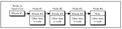
LISTING 15.1 L15-1.C
/* Deletes the node in a linked list that follows the indicated node.
Assumes list is headed by a dummy node, so no special testing for
the head-of-list pointer is required. Returns the same pointer
that was passed in. */
#include "llist.h"
struct LinkNode *DeleteNodeAfter(struct LinkNode *NodeToDeleteAfter)
{
NodeToDeleteAfter->NextNode =
NodeToDeleteAfter->NextNode->NextNode;
return(NodeToDeleteAfter);
}LISTING 15.2 LLIST.H
/* Linked list header file. */
#define MAX_TEXT_LENGTH 100 /* longest allowed Text field */
#define SENTINEL 32767 /* largest possible Value field */
struct LinkNode {
struct LinkNode *NextNode;
int Value;
char Text[MAX_TEXT_LENGTH+1];
/* Any number of additional data fields may by present */
};
struct LinkNode *DeleteNodeAfter(struct LinkNode *);
struct LinkNode *FindNodeBeforeValue(struct LinkNode *, int);
struct LinkNode *InitLinkedList(void);
struct LinkNode *InsertNodeSorted(struct LinkNode *,
struct LinkNode *);LISTING 15.3 L15-3.C
/* Deletes the node in the specified linked list that follows the
indicated node. List is headed by a head-of-list pointer; if the
pointer to the node to delete after points to the head-of-list
pointer, special handling is performed. */
#include "llist.h"
struct LinkNode *DeleteNodeAfter(struct LinkNode **HeadOfListPtr,
struct LinkNode *NodeToDeleteAfter)
{
/* Handle specially if the node to delete after is actually the
head of the list (delete the first element in the list) */
if (NodeToDeleteAfter == (struct LinkNode *)HeadOfListPtr) {
*HeadOfListPtr = (*HeadOfListPtr)->NextNode;
} else {
NodeToDeleteAfter->NextNode =
NodeToDeleteAfter->NextNode->NextNode;
}
return(NodeToDeleteAfter);
}However, it is true that if you’re going to store a variety of types
of structures in your linked lists, you should start each node with the
LinkNode field. That way, the link pointer is in the same
place in every structure, and the same linked list code can
handle all of the structure types by casting them to the base link-node
structure type. This is a less than elegant approach, but it works. C++
can handle data mixing more cleanly than C, via derivation from a base
link-node class.
Note that Listings 15.1 and 15.3 have to specify the linked-list
delete operation as “delete the next node,” rather than “delete
this node,” because in order to relink it’s necessary to access the
NextNode field of the node preceding the node to be
deleted, and it’s impossible to backtrack in a singly linked list. For
this reason, singly-linked list operations tend to work with the
structure preceding the one of interest—and that makes the problem of
having to special-case the head pointer all the more acute.
Similar problems with the head pointer crop up when you’re inserting nodes, and in fact in all link manipulation code. It’s easy to end up working with either pointers to pointers or lots of special-case code, and while those approaches work, they’re inelegant and inefficient.
Dummies and Sentinels
A far better approach is to use a dummy node for the head of the list, as shown in Figure 15.2. I invented this one for myself the next time I encountered linked lists, while designing a seed fill function for MetaWindows, back during my tenure at Metagraphics Corp. But I could have learned it by spending five minutes with Sedgewick’s book.
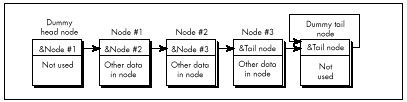
Likewise, there should be a separate node for the tail of the list,
so that every node that contains real data is guaranteed to have a node
on either side of it. In this scheme, an empty list contains two nodes,
as shown in Figure 15.3. Although it is not necessary, the tail node may
point to itself as its own next node, rather than contain a
NULL pointer. This way, a deletion operation on an empty
list will have no effect—quite unlike the same operation performed on a
list terminated with a NULL pointer. The tail node of a
list terminated like this can be detected because it will be the only
node for which the next-node pointer equals the current-node
pointer.
Figure 15.3 is a giant step in the right direction, but we can still make a few refinements. The inner loop of any code that scans through such a list has to perform a special test on each node to determine whether the tail has been reached. So, for example, code to find the first node containing a value field greater than or equal to a certain value has to perform two tests in the inner loop, as shown in Listing 15.4.
LISTING 15.4 L15-4.C
/* Finds the first node in a linked list with a value field greater
than or equal to a key value, and returns a pointer to the node
preceding that node (to facilitate insertion and deletion), or a
NULL pointer if no such value was found. Assumes the list is
terminated with a tail node pointing to itself as the next node. */
#include <stdio.h>
#include "llist.h"
struct LinkNode *FindNodeBeforeValueNotLess(
struct LinkNode *HeadOfListNode, int SearchValue)
{
struct LinkNode *NodePtr = HeadOfListNode;
while ( (NodePtr->NextNode->NextNode != NodePtr->NextNode) &&
(NodePtr->NextNode->Value < SearchValue) )
NodePtr = NodePtr->NextNode;
if (NodePtr->NextNode->NextNode == NodePtr->NextNode)
return(NULL); /* we found the sentinel; failed search */
else
return(NodePtr); /* success; return pointer to node preceding
node that was >= */
}Suppose, however, that we make the tail node a sentinel by giving it a value that is guaranteed to terminate the search, as shown in Figure 15.4. The list in Figure 15.4 has a sentinel with a value field of 32,767; since we’re working with integers, that’s the highest possible search value, and is guaranteed to satisfy any search that comes down the pike. The success or failure of the search can then be determined outside the loop, if necessary, by checking for the tail node’s special pointer—but the inside of the loop is streamlined to just one test, as shown in Listing 15.5. Not all linked lists lend themselves to sentinels, but the performance benefits are considerable for those that do.
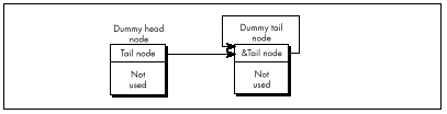
LISTING 15.5 L15-5.C
/* Finds the first node in a value-sorted linked list that
has a Value field greater than or equal to a key value, and
returns a pointer to the node preceding that node (to facilitate
insertion and deletion), or a NULL pointer if no such value was
found. Assumes the list is terminated with a sentinel tail node
containing the largest possible Value field setting and pointing
to itself as the next node. */
#include <stdio.h>
#include "llist.h"
struct LinkNode *FindNodeBeforeValueNotLess(
struct LinkNode *HeadOfListNode, int SearchValue)
{
struct LinkNode *NodePtr = HeadOfListNode;
while (NodePtr->NextNode->Value < SearchValue)
NodePtr = NodePtr->NextNode;
if (NodePtr->NextNode->NextNode == NodePtr->NextNode)
return(NULL); /* we found the sentinel; failed search */
else
return(NodePtr); /* success; return pointer to node preceding
node that was >= */
}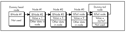
Circular Lists
One minor but elegant refinement yet remains: Use a single node as both the head and the tail of the list. We can do this by connecting the last node back to the first through the head/tail node in a circular fashion, as shown in Figure 15.5. This head/tail node can also, of course, be a sentinel; when it’s necessary to check for the end of the list explicitly, that can be done by comparing the current node pointer to the head pointer. If they’re equal, you’re at the head/tail node.
Why am I so fond of this circular list architecture? For one thing, it saves a node, and most of my linked list programming has been done in severely memory-constrained environments. Mostly, though, it’s just so neat; with this setup, there’s not a single node or inner-loop instruction wasted. Perfect economy of programming, if you ask me.
I must admit that I racked my brains for quite a while to come up with the circular list, simple as it may seem. Shortly after coming up with it, I happened to look in Sedgewick’s book, only to find my nifty optimization described plain as day; and a little while after that, I came across a thread in the algorithms/computer.sci topic on BIX that described it in considerable detail. Folks, the information is out there. Look it up before turning on your optimizer afterburners!
Listings 15.1 and 15.6 together form a suite of C functions for
maintaining a circular linked list sorted by ascending value. (Listing
15.5 requires modification before it will work with circular lists.)
Listing 15.7 is an assembly language version of
InsertNodeSorted(); note the tremendous efficiency of the
scanning loop in InsertNodeSorted()-four instructions per
node!—thanks to the dummy head/tail/sentinel node. Listing 15.8 is a
simple application that illustrates the use of the linked-list functions
in Listings 15.1 and 15.6.
Contrast Figure 15.5 with Figure 15.1, and Listings 15.1, 15.5, 15.6, and 15.7 with Listings 15.3 and 15.4. Yes, linked lists are simple, but not so simple that a little knowledge doesn’t make a substantial difference. Make it a habit to read Knuth or Sedgewick or the like before you write a single line of code.
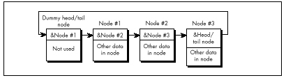
LISTING 15.6 L15-6.C
/* Suite of functions for maintaining a linked list sorted by
ascending order of the Value field. The list is circular; that
is,it has a dummy node as both the head and the tail of the list.
The dummy node is a sentinel, containing the largest possible
Value field setting. Tested with Borland C++ in C mode. */
#include <stdlib.h>
#include <stdio.h>
#include <string.h>
#include "llist.h"
/* Initializes an empty linked list of LinkNode structures,
consisting of a single head/tail/sentinel node, and returns a
pointer to the list. Returns NULL for failure. */
struct LinkNode *InitLinkedList()
{
struct LinkNode *Sentinel;
if ((Sentinel = malloc(sizeof(struct LinkNode))) == NULL)
return(NULL);
Sentinel->NextNode = Sentinel;
Sentinel->Value = SENTINEL;
strcpy(Sentinel->Text, "*** sentinel ***");
return(Sentinel);
}
/* Finds the first node in a value-sorted linked list with a value
field equal to a key value, and returns a pointer to the node
preceding that node (to facilitate insertion and deletion), or a
NULL pointer if no value was found. Assumes list is terminated
with a sentinel node containing the largest possible value. */
struct LinkNode *FindNodeBeforeValue(struct LinkNode *HeadOfListNode,
int SearchValue)
{
struct LinkNode *NodePtr = HeadOfListNode;
while (NodePtr->NextNode->Value < SearchValue)
NodePtr = NodePtr->NextNode;
if (NodePtr->NextNode->Value == SearchValue) {
/* Found the search value; success unless we found the
sentinel (can happen only if SearchValue == SENTINEL) */
if (NodePtr->NextNode == HeadOfListNode) {
return(NULL); /* failure; we found the sentinel */
} else {
return(NodePtr); /* success; return pointer to node
preceding the node that was equal */
}
} else {
return(NULL); /* No match; return failure status */
}
}
/* Inserts the specified node into a value-sorted linked list, such
that value-sorting is maintained. Returns a pointer to the node
after which the new node is inserted. */
struct LinkNode *InsertNodeSorted(struct LinkNode *HeadOfListNode,
struct LinkNode *NodeToInsert)
{
struct LinkNode *NodePtr = HeadOfListNode;
int SearchValue = NodeToInsert->Value;
while (NodePtr->NextNode->Value < SearchValue)
NodePtr = NodePtr->NextNode;
NodeToInsert->NextNode = NodePtr->NextNode;
NodePtr->NextNode = NodeToInsert;
return(NodePtr);
}LISTING 15.7 L15-7.ASM
; C near-callable assembly function for inserting a new node in a
; linked list sorted by ascending order of the Value field. The list
; is circular; that is, it has a dummy node as both the head and the
; tail of the list. The dummy node is a sentinel, containing the
; largest possible Value field setting. Tested with TASM.
MAX_TEXT_LENGTH equ 100 ;longest allowed Text field
SENTINEL equ 32767 ;largest possible Value field
LinkNode struc
NextNode dw ?
Value dw ?
Text db MAX_TEXT_LENGTH+1 dup(?)
;*** Any number of additional data fields may by present ***
LinkNode ends
.model small
.code
; Inserts the specified node into a ascending-value-sorted linked
; list, such that value-sorting is maintained. Returns a pointer to
; the node after which the new node is inserted.
; C near-callable as:
; struct LinkNode *InsertNodeSorted(struct LinkNode *HeadOfListNode,
; struct LinkNode *NodeToInsert)
parms struc
dw 2 dup (?) ;pushed return address & BP
HeadOfListNode dw ? ;pointer to head node of list
NodeToInsert dw ? ;pointer to node to insert
parms ends
public _InsertNodeSorted
_InsertNodeSorted proc near
push bp
mov bp,sp ;point to stack frame
push si ;preserve register vars
push di
mov si,[bp].NodeToInsert ;point to node to insert
mov ax,[si].Value ;search value
mov di,[bp].HeadOfListNode ;point to linked list in
; which to insert
SearchLoop:
mov bx,di ;advance to the next node
mov di,[bx].NextNode ;point to following node
cmp [di].Value,ax ;is the following node's
; value less than the value
; from the node to insert?
jl SearchLoop ;yes, so continue searching
;no, so we have found our
; insert point
mov ax,[bx].NextNode ;link the new node between
mov [si].NextNode,ax ; the current node and the
mov [bx].NextNode,si ; following node
mov ax,bx ;return pointer to node
; after which we inserted
pop di ;restore register vars
pop si
pop bp
ret
_InsertNodeSorted endp
endLISTING 15.8 L15-8.C
/* Sample linked list program. Tested with Borland C++. */
#include <stdlib.h>
#include <stdio.h>
#include <conio.h>
#include <ctype.h>
#include <string.h>
#include "llist.h"
void main()
{ int Done = 0, Char, TempValue;
struct LinkNode *TempPtr, *ListPtr, *TempPtr2;
char TempBuffer[MAX_TEXT_LENGTH+3];
if ((ListPtr = InitLinkedList()) == NULL) {
printf("Out of memory\n");
exit(1);
}
while (!Done) {
printf("\nA=add; D=delete; F=find; L=list all; Q=quit\n>");
Char = toupper(getche());
printf("\n");
switch (Char) {
case 'A': /* add a node */
if ((TempPtr = malloc(sizeof(struct LinkNode))) == NULL)
{
printf("Out of memory\n );
exit(1);
}
printf("Node value: ");
scanf("%d", &TempPtr->Value);
if ((FindNodeBeforeValue(ListPtr,TempPtr->Value))!=NULL)
{ printf("*** value already in list; try again ***\n");
free(TempPtr);
} else {printf("Node text: ");
TempBuffer[0] = MAX_TEXT_LENGTH;
cgets(TempBuffer);
strcpy(TempPtr->Text, &TempBuffer[2]);
InsertNodeSorted(ListPtr, TempPtr);
printf("\n");
}
break;
case 'D': /* delete a node */
printf("Value field of node to delete: ");
scanf("%d", &TempValue);
if ((TempPtr = FindNodeBeforeValue(ListPtr, TempValue))
!= NULL) {
TempPtr2 = TempPtr->NextNode; /* -> node to delete */
DeleteNodeAfter(TempPtr); /* delete it */
free(TempPtr2); /* free its memory */
} else {
printf("*** no such value field in list ***\n")
break;
case 'F': /* find a node */
printf("Value field of node to find: ");
scanf("%d", &TempValue);
if ((TempPtr = FindNodeBeforeValue(ListPtr, TempValue))
!= NULL)
printf("Value: %d\nText: %s\n",
TempPtr->NextNode->Value, TempPtr->NextNode->Text);
else
printf("*** no such value field in list ***\n");
break;
case 'L': /* list all nodes */
TempPtr = ListPtr->NextNode; /* point to first node */
if (TempPtr == ListPtr) { /* empty if at sentinel */
printf("*** List is empty ***\n");
} else {
do {printf("Value: %d\n Text: %s\n", TempPtr->Value,
TempPtr->Text);
TempPtr = TempPtr->NextNode;
} while (TempPtr != ListPtr);
}
break;
case 'Q':
Done = 1;
break;
default:
break;
}
}
}Hi/Lo in 24 Bytes
In one of my PC TECHNIQUES “Pushing the Envelope” columns, I
passed along one of David Stafford’s fiendish programming puzzles: Write
a C-callable function to find the greatest or smallest unsigned
int. Not a big deal—except that David had already
done it in 24 bytes, so the challenge was to do it in 24 bytes or
less.
Such routines soon began coming at me from all angles. However (and I
hate to say this because some of my correspondents were very
pleased with the thought that they had bested David), no one has yet met
the challenge—because most of you folks missed a key point. When David
said, “Write a function to find the greatest or smallest unsigned
int in 24 bytes or less,” he meant, “Write the
hi and the lo functions in 24 bytes or
less—combined.”
Oh.
Yes, a 24-byte hi/lo function is possible, anatomically improbable as it might seem. Which I guess goes to show that when one of David’s puzzles seems less than impossible, odds are you’re missing something. Listing 15.9 is David’s 24-byte solution, from which a lot may be learned if one reads closely enough.
LISTING 15.9 L15-9.ASM
; Find the greatest or smallest unsigned int.
; C callable (small model); 24 bytes.
; By David Stafford.
; unsigned hi( int num, unsigned a[] );
; unsigned lo( int num, unsigned a[] );
public _hi, _lo
_hi: db 0b9h ;mov cx,immediate
_lo: xor cx,cx
pop ax ;get return address
pop dx ;get count
pop bx ;get pointer
push bx ;restore pointer
push dx ;restore count
push ax ;restore return address
save: mov ax,[bx]
top: cmp ax,[bx]
jcxz around
cmc
around: ja save
inc bx
inc bx
dec dx
jnz top
retBefore I end this chapter, let me say that I get a lot of feedback from my readers, and it’s much appreciated. Keep those cards, letters, and email messages coming. And if any of you know Jeannie Schweigert, have her drop me a line and let me know how she’s doing these days….
Chapter 16 – There Ain’t No Such Thing as the Fastest Code
Lessons Learned in the Pursuit of the Ultimate Word Counter
I remember reading an overview of C++ development tools for Windows in a past issue of PC Week. In the lower left corner was the familiar box listing the 10 leading concerns of corporate buyers when it comes to C++. Boiled down, the list looked like this, in order of descending importance to buyers:
Debugging
Documentation
Windows development tools
High-level Windows support
Class library
Development cycle efficiency
Object-oriented development aids
Programming management aids
Online help
10. Windows development cycle automation
Is something missing here? You bet your maximum gluteus something’s missing—nowhere on that list is there so much as one word about how fast the compiled code runs! I’m not saying that performance is everything, but optimization isn’t even down there at number 10, below online help! Ye gods and little fishes! We are talking here about people who would take a bus from LA to New York instead of a plane because it had a cleaner bathroom; who would choose a painting from a Holiday Inn over a Matisse because it had a fancier frame; who would buy a Yugo instead of—well, hell, anything—because it had a nice owner’s manual and particularly attractive keys. We are talking about people who are focusing on means, and have forgotten about ends. We are talking about people with no programming souls.
Counting Words in a Hurry
What are we to make of this? At the very least, we can safely guess that very few corporate buyers ever enter optimization contests. Most of my readers do, however; in fact, far more than I thought ever would, but that gladdens me to no end. I issued my first optimization challenge in a “Pushing the Envelope” column in PC TECHNIQUES back in 1991, and was deluged by respondents who, one might also gather, do not live by PC Week.
That initial challenge was sparked by a column David Gerrold wrote (also in PC TECHNIQUES ) concerning the matter of counting the number of words in a document; David turned up some pretty interesting optimization issues along the way. David did all his coding in Pascal, pointing out that while an assembly language version would probably be faster, his Pascal utility worked properly and was fast enough for him.
It wasn’t, however, fast enough for me. The logical starting place for speeding up word counting would be David’s original Pascal code, but I’m much more comfortable with C, so Listing 16.1 is a loose approximation of David’s word count program, translated to C. I left out a few details, such as handling comment blocks, partly because I don’t use such blocks myself, and partly so we can focus on optimizing the core word-counting code. As Table 16.1 indicates, Listing 16.1 counts the words in a 104,448-word file in 4.6 seconds. The file was stored on a RAM disk, and Listing 16.1 was compiled with Borland C++ with all optimization enabled. A RAM disk was used partly because it returns consistent times—no seek times, rotational latency, or cache to muddy the waters—and partly to highlight word-counting speed rather than disk access speed.
| Listing | Time to Count Words |
|---|---|
| 16.1 (C) | 4.6 seconds |
| 16.2 & 16.3 (C+ASM) | 2.4 seconds |
| 16.2 & 16.4 (C+ASM w/lookup) | 1.6 seconds |
These are the times taken to search a file containing 104,448 words, timed from a RAM disk on a 20 MHz 386.
LISTING 16.1 L16-1.C
/* Word-counting program. Tested with Borland C++ in C
compilation mode and the small model. */
#include <stdio.h>
#include <fcntl.h>
#include <sys\stat.h>
#include <stdlib.h>
#include <io.h>
#define B UFFER_SIZE 0x8000 /* largest chunk of file worked
with at any one time */
int main(int, char **);
int main(int argc, char **argv) {
int Handle;
unsigned int BlockSize;
long FileSize;
unsigned long WordCount = 0;
char *Buffer, CharFlag = 0, PredCharFlag, *BufferPtr, Ch;
if (argc != 2) {
printf("usage: wc <filename>\n");
exit(1);
}
if ((Buffer = malloc(BUFFER_SIZE)) == NULL) {
printf("Can't allocate adequate memory\n");
exit(1);
}
if ((Handle = open(argv[1], O_RDONLY | O_BINARY)) == -1) {
printf("Can't open file %s\n", argv[1]);
exit(1);
}
if ((FileSize = filelength(Handle)) == -1) {
printf("Error sizing file %s\n", argv[1]);
exit(1);
}
/* Process the file in chunks */
while (FileSize > 0) {
/* Get the next chunk */
FileSize -= (BlockSize = min(FileSize, BUFFER_SIZE));
if (read(Handle, Buffer, BlockSize) == -1) {
printf("Error reading file %s\n", argv[1]);
exit(1);
}
/* Count words in the chunk */
BufferPtr = Buffer;
do {
PredCharFlag = CharFlag;
Ch = *BufferPtr++ & 0x7F; /* strip high bit, which some
word processors set as an
internal flag */
CharFlag = ((Ch >= 'a') && (Ch <= 'z')) ||
((Ch >= 'A') && (Ch <= 'Z')) ||
((Ch >= '0') && (Ch <= '9')) ||
(Ch == '\'');
if ((!CharFlag) && PredCharFlag) {
WordCo u nt++;
}
} while (—BlockSize);
}
/* Catch the last word, if any */
if (CharFlag) {
WordCount++;
}
printf("\nTotal words in file: %lu\n", WordCount);
return(0);
}Listing 16.2 is Listing 16.1 modified to call a function that scans each block for words, and Listing 16.3 contains an assembly function that counts words. Used together, Listings 16.2 and 16.3 are just about twice as fast as Listing 16.1, a good return for a little assembly language. Listing 16.3 is a pretty straightforward translation from C to assembly; the new code makes good use of registers, but the key code—determining whether each byte is a character or not—is still done with the same multiple-sequential-tests approach used by the code that the C compiler generates.
LISTING 16.2 L16-2.C
/* Word-counting program incorporating assembly language. Tested
with Borland C++ in C compilation mode & the small model. */
#include <stdio.h>
#include <fcntl.h>
#include <sys\stat.h>
#include <stdlib.h>
#include <io.h>
#define BUFFER_SIZE 0x8000 /* largest chunk of file worked
with at any one time */
int main(int, char **);
void ScanBuffer(char *, unsigned int, char *, unsigned long *);
int main(int argc, char **argv) {
int Handle;
unsigned int BlockSize;
long FileSize;
unsigned long WordCount = 0;
char *Buffer, CharFlag = 0;
if (argc != 2) {
printf("usage: wc <filename>\n");
exit(1);
}
if ((Buffer = malloc(BUFFER_SIZE)) == NULL) {
printf("Can't allocate adequate memory\n");
exit(1);
}
if ((Handle = open(argv[1], O_RDONLY | O_BINARY)) == -1) {
printf("Can't open file %s\n", argv[1]);
exit(1);
}
if ((FileSize = filelength(Handle)) == -1) {
printf("Error sizing file %s\n", argv[1]);
exit(1);
}
CharFlag = 0;
while (FileSize > 0) {
FileSize -= (BlockSize = min(FileSize, BUFFER_SIZE));
if (read(Handle, Buffer, BlockSize) == -1) {
printf("Error reading file %s\n", argv[1]);
exit(1);
}
ScanBuffer(Buffer, BlockSize, &CharFlag, &WordCount);
}
/* Catch the last word, if any */
if (CharFlag) {
WordCount++;
}
printf("\nTotal words in file: %lu\n", WordCount);
return(0);
}LISTING 16.3 L16-3.ASM
; Assembly subroutine for Listing 16.2. Scans through Buffer, of
; length BufferLength, counting words and updating WordCount as
; appropriate. BufferLength must be > 0. *CharFlag and *WordCount
; should equal 0 on the first call. Tested with TASM.
; C near-callable as:
; void ScanBuffer(char *Buffer, unsigned int BufferLength,
; char *CharFlag, unsigned long *WordCount);
parms struc
dw 2 dup(?) ;pushed return address & BP
Buffer dw ? ;buffer to scan
BufferLength dw ? ;length of buffer to scan
CharFlag dw ? ;pointer to flag for state of last
; char processed on entry (0 on
; initial call). Updated on exit
WordCount dw ? ;pointer to 32-bit count of words
; found (0 on initial call)
parms ends
.model small
.code
public _ScanBuffer
_ScanBuffer proc near
push bp ;preserve caller's stack frame
mov bp,sp ;set up local stack frame
push si ;preserve caller's register vars
push di
mov si,[bp+Buffer] ;point to buffer to scan
mov bx,[bp+WordCount]
mov cx,[bx] ;get current 32-bit word count
mov dx,[bx+2]
mov bx,[bp+CharFlag]
mov bl,[bx] ;get current CharFlag
mov di,[bp+BufferLength];get # of bytes to scan
ScanLoop:
mov bh,bl ;PredCharFlag = CharFlag;
lodsb ;Ch = *BufferPtr++ & 0x7F;
and al,7fh ;strip high bit for word processors
; that set it as an internal flag
mov bl,1 ;assume this is a char; CharFlag = 1;
cmp al,'a' ;it is a char if between a and z
jb CheckAZ
cmp al,'z'
jna IsAChar
CheckAZ:
cmp al,'A' ;it is a char if between A and Z
jb Check09
cmp al,'Z'
jna IsAChar
Check09:
cmp al,'0' ;it is a char if between 0 and 9
jb CheckApostrophe
cmp al,'9'
jna IsAChar
CheckApostrophe:
cmp al,27h ;it is a char if an apostrophe
jz IsAChar
sub bl,bl ;not a char; CharFlag = 0;
and bh,bh
jz ScanLoopBottom ;if ((!CharFlag) && PredCharFlag) {
add cx,1 ; (WordCount)++;
adc dx,0 ;}
IsAChar:
ScanLoopBottom:
dec di ;} while (—BufferLength);
jnz ScanLoop
mov si,[bp+CharFlag]
mov [si],bl ;set new CharFlag
mov bx,[bp+WordCount]
mov [bx],cx ;set new word count
mov [bx+2],dx
pop di ;restore caller's register vars
pop si
pop bp ;restore caller's stack frame
ret
_ScanBuffer endp
endWhich Way to Go from Here?
We could rearrange the tests in light of the nature of the data being scanned; for example, we could perform the tests more efficiently by taking advantage of the knowledge that if a byte is less than ‘0,’ it’s either an apostrophe or not a character at all. However, that sort of fine-tuning is typically good for speedups of only 10 to 20 percent, and I’ve intentionally refrained from implementing this in Listing 16.3 to avoid pointing you down the wrong path; what we need is a different tack altogether. Ponder this. What we really want to know is nothing more than whether a byte is a character, not what sort of character it is. For each byte value, we want a yes/no status, and nothing else—and that description practically begs for a lookup table. Listing 16.4 uses a lookup table approach to boost performance another 50 percent, to three times the performance of the original C code. On a 20 MHz 386, this represents a change from 4.6 to 1.6 seconds, which could be significant—who likes to wait? On an 8088, the improvement in word-counting a large file could easily be 10 or 20 seconds, which is definitely significant.
LISTING 16.4 L16-4.ASM
; Assembly subroutine for Listing 16.2. Scans through Buffer, of
; length BufferLength, counting words and updating WordCount as
; appropriate, using a lookup table-based approach. BufferLength
; must be > 0. *CharFlag and *WordCount should equal 0 on the
; first call. Tested with TASM.
; C near-callable as:
; void ScanBuffer(char *Buffer, unsigned int BufferLength,
; char *CharFlag, unsigned long *WordCount);
parms struc
dw 2 dup(?) ;pushed return address & BP
Buffer dw ? ;buffer to scan
BufferLength dw ? ;length of buffer to scan
CharFlag dw ? ;pointer to flag for state of last
;char processed on entry (0 on
;initial call). Updated on exit
WordCount dw ? ;pointer to 32-bit count of words
; found (0 on initial call)
parms ends
.model small
.data
; Table of char/not statuses for byte values 0-255 (128-255 are
; duplicates of 0-127 to effectively mask off bit 7, which some
; word processors set as an internal flag).
CharStatusTable label byte
REPT 2
db 39 dup(0)
db 1 ;apostrophe
db 8 dup(0)
db 10 dup(1) ;0-9
db 7 dup(0)
db 26 dup(1) ;A-Z
db 6 dup(0)
db 26 dup(1) ;a-z
db 5 dup(0)
ENDM
.code
public _ScanBuffer
_ScanBuffer proc near
push bp ;preserve caller's stack frame
mov bp,sp ;set up local stack frame
push si ;preserve caller's register vars
push di
mov si,[bp+Buffer] ;point to buffer to scan
mov bx,[bp+WordCount]
mov di,[bx] ;get current 32-bit word count
mov dx,[bx+2]
mov bx,[bp+CharFlag]
mov al,[bx] ;get current CharFlag
mov cx,[bp+BufferLength] ;get # of bytes to scan
mov bx,offset CharStatusTable
ScanLoop:
and al,al ;ZF=0 if last byte was a char,
; ZF=1 if not
lodsb ;get the next byte
;***doesn't change flags***
xlat ;look up its char/not status
;***doesn't change flags***
jz ScanLoopBottom ;don't count a word if last byte was
; not a character
and al,al ;last byte was a character; is the
; current byte a character?
jz CountWord ;no, so count a word
ScanLoopBottom:
dec cx ;count down buffer length
jnz ScanLoop
Done:
mov si,[bp+CharFlag]
mov [si],al ;set new CharFlag
mov bx,[bp+WordCount]
mov [bx],di ;set new word count
mov [bx+2],dx
pop di ;restore caller's register vars
pop si
pop bp ;restore caller's stack frame
ret
align 2
CountWord:
add di,1 ;increment the word count
adc dx,0
dec cx ;count down buffer length
jnz ScanLoop
jmp Done
_ScanBuffer endp
endListing 16.4 features several interesting tricks. First, it uses
LODSB and XLAT in succession, a very neat way
to get a pointed-to byte, advance the pointer, and look up the value
indexed by the byte in a table, all with just two instruction bytes.
(Interestingly, Listing 16.4 would probably run quite a bit better still
on an 8088, where LODSB and XLAT have a
greater advantage over conventional instructions. On the 486 and
Pentium, however, LODSB and XLAT lose much of
their appeal, and should be replaced with MOV
instructions.) Better yet, LODSB and XLAT
don’t alter the flags, so the Zero flag status set before
LODSB is still around to be tested after XLAT
.
Finally, if you look closely, you will see that Listing 16.4 jumps out of the loop to increment the word count in the case where a word is actually found, with a duplicate of the loop-bottom code placed after the code that increments the word count, to avoid an extra branch back into the loop; this replaces the more intuitive approach of jumping around the incrementing code to the loop bottom when a word isn’t found. Although this incurs a branch every time a word is found, a word is typically found only once every 5 or 6 bytes; on average, then, a branch is saved about two-thirds of the time. This is an excellent example of how understanding the nature of the data you’re processing allows you to optimize in ways the compiler can’t. Know your data!
So, gosh, Listing 16.4 is the best word-counting code in the universe, right? Not hardly. If there’s one thing my years of toil in this vale of silicon have taught me, it’s that there’s never a lack of potential for further optimization. Never! Off the top of my head, I can think of at least three ways to speed up Listing 16.4; and, since Turbo Profiler reports that even in Listing 16.4, 88 percent of the time is spent scanning the buffer (as opposed to reading the file), there’s potential for those further optimizations to improve performance significantly. (However, it is true that when access is performed to a hard rather than RAM disk, disk access jumps to about half of overall execution time.) One possible optimization is unrolling the loop, although that is truly a last resort because it tends to make further changes extremely difficult.
Challenges and Hazards
The challenge I put to the readers of PC TECHNIQUES was to write a faster module to replace Listing 16.4. The author of the code that counted the words in my secret test file fastest on my 20 MHz cached 386 would be the winner and receive Numerous Valuable Prizes.
No listings were to be longer than 200 lines. No complete programs were to be accepted; submissions had to be plug-compatible with Listing 16.4. (This was to encourage people not to waste time optimizing outside the inner loop.) Finally, the code had to produce the same results as Listing 16.4; I didn’t want to see functions that approximated the word count by dividing the number of characters by six instead of counting actual words!
So how did the entrants in this particular challenge stack up? More than one claimed a speed-up over my assembly word-counting code of more than three times. On top of the three-times speedup over the original C code that I had already realized, we’re almost up to an order of magnitude faster. You are, of course, entitled to your own opinion, but I consider an order of magnitude to be significant.
Truth to tell, I didn’t expect a three-times speedup; around two times was what I had in mind. Which just goes to show that any code can be made faster than you’d expect, if you think about it long enough and from many different perspectives. (The most potent word-counting technique seems to be a 64K lookup table that allows handling two bytes simultaneously. This is not the sort of technique one comes up with by brute-force optimization.) Thinking (or, worse yet, boasting) that your code is the fastest possible is rollescating on a tightrope in a hurricane; you’re due for a fall, if you catch my drift. Case in point: Terje Mathisen’s word-counting program.
Blinding Yourself to a Better Approach
Not so long ago, Terje Mathisen, who I introduced earlier in this book, wrote a very fast word-counting program, and posted it on Bix. When I say it was fast, I mean fast; this code was optimized like nobody’s business. We’re talking top-quality code here.
When the topic of optimizing came up in one of the Bix conferences, Terje’s program was mentioned, and he posted the following message: “I challenge BIXens (and especially mabrash!) to speed it up significantly. I would consider 5 percent a good result.” The clear implication was, “That code is as fast as it can possibly be.”
Naturally, it wasn’t; there ain’t no such thing as the fastest code (TANSTATFC? I agree, it doesn’t have the ring of TANSTAAFL). I pored over Terje’s 386 native-mode code, and found the critical inner loop, which was indeed as tight as one could imagine, consisting of just a few 386 native-mode instructions. However, one of the instructions was this:
CMP DH,[EBX+EAX]Harmless enough, save for two things. First, EBX happened to be zero
at this point (a leftover from an earlier version of the code, as it
turned out), so it was superfluous as a memory-addressing component;
this made it possible to use base-only addressing ([EAX])
rather than base+index addressing ([EBX+EAX]), which saves
a cycle on the 386. Second: Changing the instruction to
CMP [EAX],DH saved 2 cycles—just enough, by good fortune,
to speed up the whole program by 5 percent.
CMP reg,[mem]takes 6 cycles on the 386, butCMP [ mem ],regtakes only 5 cycles; you should always performCMPwith the memory operand on the left on the 386.
(Granted, CMP [*mem*],*reg* is 1 cycle slower than
CMP *reg*,[*mem*] on the 286, and they’re both the same on
the 8088; in this case, though, the code was specific to the 386. In
case you’re curious, both forms take 2 cycles on the 486; quite a lot
faster, eh?)
Watch Out for Luggable Assumptions!
The first lesson to be learned here is not to lug assumptions that
may no longer be valid from the 8088/286 world into the wonderful new
world of 386 native-mode programming. The second lesson is that after
you’ve slaved over your code for a while, you’re in no shape to see its
flaws, or to be able to get the new perspectives needed to speed it up.
I’ll bet Terje looked at that [EBX+EAX] addressing a
hundred times while trying to speed up his code, but he didn’t really
see what it did; instead, he saw what it was supposed to do. Mental
shortcuts like this are what enable us to deal with the complexities of
assembly language without overloading after about 20 instructions, but
they can be a major problem when looking over familiar code.
The third, and most interesting, lesson is that a far more fruitful optimization came of all this, one that nicely illustrates that cycle counting is not the key to happiness, riches, and wondrous performance. After getting my 5 percent speedup, I mentioned to Terje the possibility of using a 64K lookup table. (This predated the arrival of entries for the optimization contest.) He said that he had considered it, but it didn’t seem to him to be worthwhile. He couldn’t shake the thought, though, and started to poke around, and one day, voila, he posted a new version of his word count program, WC50, that was much faster than the old version. I don’t have exact numbers, but Terje’s preliminary estimate was 80 percent faster, and word counting—including disk cache access time—proceeds at more than 3 MB per second on a 33 MHz 486. Even allowing for the speed of the 486, those are very impressive numbers indeed.
The point I want to make, though, is that the biggest optimization barrier that Terje faced was that he thought he had the fastest code possible. Once he opened up the possibility that there were faster approaches, and looked beyond the specific approach that he had so carefully optimized, he was able to come up with code that was a lot faster. Consider the incongruity of Terje’s willingness to consider a 5 percent speedup significant in light of his later near-doubling of performance.
By the way, Terje’s WC50 program is a full-fledged counting program; it counts characters, words, and lines, can handle multiple files, and lets you specify the characters that separate words, should you so desire. Source code is provided as part of the archive WC50 comes in. All in all, it’s a nice piece of work, and you might want to take a look at it if you’re interested in really fast assembly code. I wouldn’t call it the fastest word-counting code, though, because I would of course never be so foolish as to call anything the fastest.
The Astonishment of Right-Brain Optimization
As it happened, the challenge I issued to my PC TECHNIQUES readers was a smashing success, with dozens of good entries. I certainly enjoyed it, even though I did have to look at a lot of tricky assembly code that I didn’t write—hard work under the best of circumstances. It was worth the trouble, though. The winning entry was an astonishing example of what assembly language can do in the right hands; on my 386, it was four times faster at word counting than the nice, tight assembly code I provided as a starting point—and about 13 times faster than the original C implementation. Attention, high-level language chauvinists: Is the speedup getting significant yet? Okay, maybe word counting isn’t the most critical application, but how would you like to have that kind of improvement in your compression software, or in your real-time games—or in Windows graphics?
The winner was David Stafford, who at the time was working for Borland International; his entry is shown in Listing 16.5. Dave Methvin, whom some of you may recall as a tech editor of the late, lamented PC Tech Journal, was a close second, and Mick Brown, about whom I know nothing more than that he is obviously an extremely good assembly language programmer, was a close third, as shown in Table 16.2, which precedes Listing 16.5. Those three were out ahead of the pack; the fourth-place entry, good as it was (twice as fast as my original code), was twice as slow as David’s winning entry, so you can see that David, Dave, and Mick attained a rarefied level of optimization indeed.
Table 16.2 has two times for each entry listed: the first value is
the overall counting time, including time spent in the main program,
disk I/O, and everything else; the second value is the time actually
spent counting words, the time spent in ScanBuffer . The
first value is the time perceived by the user, but the second value best
reflects the quality of the optimization in each entry, since the rest
of the overall execution time is fixed.
Word-Counting Time
| Name | Overall time | (ScanBuffer only) |
|---|---|---|
| David Stafford Listing 16.5 | 0.61 seconds | 0.33 seconds |
| Dave Methvin | 0.66 | 0.39 |
| Mick Brown | 0.70 | 0.41 |
| Wendell Neubert | 0.92 | 0.65 |
| For Comparison: | ||
| Michael Abrash assembly code Listing 16.1 | 1.73 | 1.44 |
| Michael Abrash C code Listing 16.4 | 4.70 | 4.43 |
Note: All times measured on a 20 MHz cached 386 DX.
LISTING 16.5 QSCAN3.ASM
; QSCAN3.ASM
; David Stafford
COMMENT $
How it works
——————
The idea is to go through the buffer fetching each letter-pair (words
rather than bytes). The carry flag indicates whether we are
currently in a (text) word or not. The letter-pair fetched from the
buffer is converted to a 16-bit address by shifting it left one bit
(losing the high bit of the second character) and putting the carry
flag in the low bit. The high bit of the count register is set to
1. Then the count register is added to the byte found at the given
address in a large (64K, naturally) table. The byte at the given
address will contain a 1 in the high bit if the last character of the
letter-pair is a word-letter (alphanumeric or apostrophe). This will
set the carry flag since the high bit of the count register is also a
1. The low bit of the byte found at the given address will be one if
the second character of the previous letter-pair was a word-letter
and the first character of this letter-pair is not a word-letter. It
will also be 1 if the first character of this letter-pair is a
word-letter but the second character is not. This process is
repeated. Finally, the carry flag is saved to indicate the final
in-a-word/not-in-a-word status. The count register is masked to
remove the high bit and the count of words remains in the count
register.
Sound complicated? You're right! But it's fast!
The beauty of this method is that no jumps are required, the
operations are fast, it requires only one table and the process can
be repeated (unrolled) many times. QSCAN3 can read 256 bytes without
jumping.
COMMEND $
.model small
.code
Test1 macro x,y ;9 or 10 bytes
Addr&x: mov di,[bp+y] ;3 or 4 bytes
adc di,di
or ax,si
add al,[di]
endm
Test2 macro x,y ;7 or 8 bytes
Addr&x: mov di,[bp+y] ;3 or 4 bytes
adc di,di
add ah,[di]
endm
Scan = 128 ;scan 256 bytes at a time
Buffer = 4 ;parms
BufferLength = 6
CharFlag = 8
WordCount = 10
public _ScanBuffer
_ScanBuffer proc near
push bp
mov bp,sp
push si
push di
xor cx,cx
mov si,[bp+Buffer] ;si = text buffer
mov ax,[bp+BufferLength] ;dx = length in bytes
shr ax,1 ;dx = length in words
jnz NormalBuf
OneByteBuf:
mov ax,seg WordTable
mov es,ax
mov di,[bp+CharFlag]
mov bh,[di] ;bh = old CharFlag
mov bl,[si] ;bl = character
add bh,'A'-1 ;make bh into character
add bx,bx ;prepare to index
mov al,es:[bx]
cbw ;get hi bit in ah (then bh)
shr al,1 ;get low bit
adc cx,cx ;cx = 0 or 1
xchg ax,bx
jmp CleanUp
NormalBuf:
push bp ;(1)
pushf ;(2)
cwd ;dx = 0
mov cl,Scan
div cx
or dx,dx ;remainder?
jz StartAtTheTop ;nope, do the whole banana
sub cx,dx
sub si,cx ;adjust buf pointer
sub si,cx
inc ax ;adjust for partial read
StartAtTheTop: mov bx,dx ;get index for start...
shl bx,1
mov di,LoopEntry[bx] ;...address in di
xchg dx,ax ;dx is the loop counter
xor cx,cx ;total word count
mov bx,[bp+CharFlag]
mov bl,[bx] ;bl = old CharFlag
mov bp,seg WordTable
mov ds,bp
mov bp,si ;scan buffer with bp
mov si,8080h ;hi bits
mov ax,si ;init local word counter
shr bl,1 ;carry = old CharFlag
jmp di
align 2
Top: add bx,bx ;restore carry
n = 0
rept Scan/2
Test1 %n,%n*2
Test2 %n+1,%n*2+2
n = n+2
endm
EndCount:
sbb bx,bx ;save carry
if Scan ge 128 ;because al+ah may equal 128!
or ax,si
add al,ah
mov ah,0
else
add al,ah
and ax,7fh ;mask
endif
add cx,ax ;update word count
mov ax,si
add bp,Scan*2
dec dx ;any left?
jng Quit
jmp Top
Quit: popf ;(2) even or odd buffer?
jnc ItsEven
clc
Test1 Odd,-1
sbb bx,bx ;save carry
shr ax,1
adc cx,0
ItsEven:
push ss ;restore ds
pop ds
pop bp ;(1)
CleanUp:
mov si,[bp+WordCount]
add [si],cx
adc word ptr [si+2],0
and bh,1 ;save only the carry flag
mov si,[bp+CharFlag]
mov [si],bh
pop di
pop si
pop bp
ret
_ScanBuffer endp
.data
Address macro X
dw Addr&X
endm
LoopEntry label word
n = Scan
REPT Scan
Address %n MOD Scan
n = n - 1
ENDM
.fardata WordTable
include qscan3.inc ;built by MAKETAB
endLevels of Optimization
Three levels of optimization were evident in the word-counting entries I received in response to my challenge. I’d briefly describe them as “fine-tuning,” “new perspective,” and “table-driven state machine.” The latter categories produce faster code, but, by the same token, they are harder to design, harder to implement, and more difficult to understand, so they’re suitable for only the most demanding applications. (Heck, I don’t even guarantee that David Stafford’s entry works perfectly, although, knowing him, it probably does; the more complex and cryptic the code, the greater the chance for obscure bugs.)
Optimization Level 1: Good Code
The first level of optimization involves fine-tuning and clever use of the instruction set. The basic framework is still the same as my code (which in turn is basically the same as that of the original C code), but that framework is implemented more efficiently.
One obvious level 1 optimization is using a word rather
than dword counter. ScanBuffer can never be
called upon to handle more than 64K bytes at a time, so no more than 32K
words can ever be found. Given that, it’s a logical step to use
INC rather than ADD/ADC to keep count, adding
the tally into the full 32-bit count only upon exiting the function.
Another useful optimization is aligning loop tops and other branch
destinations to word , or better yet dword ,
boundaries.
Eliminating branches was very popular, as it should be on x86
processors. Branches were eliminated in a remarkable variety of ways.
Many of you unrolled the loop, a technique that does pay off nicely. A
word of caution: Some of you unrolled the loop by simply stacking
repetitions of the inner loop one after the other, with
DEC CX/JZ appearing after each repetition to detect the end
of the buffer. Part of the point of unrolling a loop is to reduce the
number of times you have to check for the end of the buffer! The trick
to this is to set CX to the number of repetitions of the
unrolled loop and count down only once each time through the
unrolled loop. In order to handle repetition counts that aren’t exact
multiples of the unrolling factor, you must enter the loop by branching
into the middle of it to perform whatever fraction of the number of
unrolled repetitions is required to make the whole thing come out right.
Listing 16.5 (QSCAN3.ASM) illustrates this technique.
Another effective optimization is the use of LODSW
rather than LODSB , thereby processing two bytes per memory
access. This has the effect of unrolling the loop one time, since with
LODSW , looping is performed at most only once every two
bytes.
Cutting down the branches used to loop is only part of the branching story. More often than not, my original code also branched in the process of checking whether it was time to count a word. There are many ways to reduce this sort of branching; in fact, it is quite possible to eliminate it entirely. The most straightforward way to reduce such branching is to employ two loops. One loop is used to look for the end of a word when the last byte was a non-separator, and one loop is used to look for the start of a word when the last byte was a separator. This way, it’s no longer necessary to maintain a flag to indicate the state of the last byte; that state is implied by whichever loop is currently executing. This considerably simplifies and streamlines the inner loop code.
Listing 16.6, contributed by Willem Clements, of Granada, Spain,
illustrates a variety of level 1 optimizations: the two-loop approach,
the use of a 16- rather than 32-bit counter, and the use of
LODSW . Together, these optimizations made Willem’s code
nearly twice as fast as mine in Listing 16.4. A few details could stand
improvement; for example, AND AX,AX is a shorter way to
test for zero than CMP AX,0 , and ALIGN 2
could be used. Nonetheless, this is good code, and it’s also fairly
compact and reasonably easy to understand. In short, this is an
excellent example of how an hour or so of hand-optimization might
accomplish significantly improved performance at a reasonable cost in
complexity and time. This level of optimization is adequate for most
purposes (and, in truth, is beyond the abilities of most
programmers).
Listing 16.6 OPT2.ASM
;
; Opt2 Final optimization word count
; Written by Michael Abrash
; Modified by Willem Clements
; C/ Moncayo 5, Laurel de la Reina
; 18140 La Zubia
; Granada, Spain
; Tel 34-58-890398
; Fax 34-58-224102
;
parms struc
dw 2 dup(?)
buffer dw ?
bufferlength dw ?
charflag dw ?
wordcount dw ?
parms ends
.model small
.data
charstatustable label byte
rept 2
db 39 dup(0)
db 1
db 8 dup(0)
db 10 dup(1)
db 7 dup(0)
db 26 dup(1)
db 6 dup(0)
db 26 dup(1)
db 5 dup(0)
endm
.code
public _ScanBuffer
_ScanBuffer proc near
push bp
mov bp,sp
push si
push di
mov si,[bp+buffer]
mov bx,[bp+charflag]
mov al,[bx]
mov cx,[bp+bufferlength]
mov bx,offset charstatustable
xor di,di ; set wordcount to zero
shr cx,1 ; change count to wordcount
jc oddentry ; odd number of bytes to process
cmp al,01h ; check if last one is char
jne scanloop4 ; if not so, search for char
jmp scanloop1 ; if so, search for zero
oddentry: xchg al,ah ; last one in ah
lodsb ; get first byte
inc cx
cmp ah,01h ; check if last one was char
jne scanloop5 ; if not so, search for char
jmp scanloop2 ; if so, search for zero
;
; locate the end of a word
scanloop1: lodsw ; get two chars
xlat ; translate first
xchg al,ah ; first in ah
scanloop2: xlat ; translate second
dec cx ; count down
jz done1 ; no more bytes left
cmp ax,0101h ; check if two chars
je scanloop1 ; go for next two bytes
inc di ; increase wordcount
cmp al,01h ; check if new word started
je scanloop1 ; locate end of word
;
; locate the begin of a word
scanloop4: lodsw ; get two chars
xlat ; translate first
xchg al,ah ; first in ah
scanloop5: xlat ; translate second
dec cx ; count down
jz done2 ; no more bytes left
cmp ax,0 ; check if word started
je scanloop4 ; if not, locate begin
cmp al,01h ; check one-letter word
je scanloop1 ; if not, locate end of word
inc di ; increase wordcount
jmp scanloop4 ; locate begin of next word
done1: cmp ax,0101h ; check if end-of-word
je done ; if not, we have finished
inc di ; increase wordcount
jmp done
done2: cmp ax,0100h ; check for one-letter word
jne done ; if not, we have finished
inc di ; increase wordcount
done: mov si,[bp+charflag]
mov [si],al
mov bx,[bp+wordcount]
mov ax,[bx]
mov dx,[bx+2]
add di,ax
adc dx,0
mov [bx],di
mov [bx+2],dx
pop di
pop si
pop bp
ret
_ScanBuffer endp
endLevel 2: A New Perspective
The second level of optimization is one of breaking out of the mode of thinking established by my original code. Some entrants clearly did exactly that. They stepped back, thought about what the code actually needed to do, rather than just improving how it already worked, and implemented code that sprang from that new perspective.
You can see one example of this in Listing 16.6, where Willem uses
CMP AX,0101H to check two bytes at once. While you might
think of this as nothing more than a doubling up of tests, it’s a little
more than that, especially when taken together with the use of two
loops. This is a break with the serial nature of the C code, a
recognition that word counting is really nothing more than a state
machine that transitions from the “in word” state to the “not in word”
state and back, counting a word on one but not both of those
transitions. Willem says, in effect, “We’re in a word; if the next two
bytes are non-separators, then we’re still in a word, else we’re not in
a word, so count and change to the appropriate state.” That’s really
quite different from saying, as I originally did, “If the last byte was
a non-separator, then if the current byte is a separator, then count a
word.” Willem has moved away from the all-in-one approach, splitting the
code up into state-specific chunks that are more efficient because each
does only the work required in a particular state.
Another example of coming at the code from a new perspective is counting a word as soon as a non-separator follows a separator (at the start of the word), rather than waiting for a separator following a non-separator (at the end of the word). My friend Dan Illowsky describes the thought process leading to this approach thusly:
“I try to code as closely as possible to the real world nature of
those things my program models. It seems somehow wrong to me to count
the end of a word as you do when you look for a transition from a word
to a non-word. A word is not a transition, it is the presence of a group
of characters. Thought of this way, the code would have counted the word
when it first detected the group. Had you done this, your main program
would not have needed to look for the possible last transition or deal
with the semantics of the value in CharValue.”
John Richardson, of New York, contributed a good example of the benefits of a different perspective (in this case, a hardware perspective). John eliminated all branches used for detecting word edges; the inner loop of his code is shown in Listing 16.7. As John explains it:
“My next shot was to get rid of all the branches in the loop. To do that, I reached back to my college hardware courses. I noticed that we were really looking at an edge triggered device we want to count each time the I’m a character state goes from one to zero. Remembering that XOR on two single-bit values will always return whether the bits are different or the same, I implemented a transition counter. The counter triggers every time a word begins or ends.”
Listing 16.7 L16-7.ASM
ScanLoop:
lodsw ;get the next 2 bytes (AL = first, AH = 2nd)
xlat ;look up first's char/not status
xor dl,al ;see if there's a new char/not status
add di,dx ;we add 1 for each char/not transition
mov dl,al
mov al,ah ;look at the second byte
xlat ;look up its char/not status
xor dl,al ;see if there's a new char/not status
add di,dx ;we add 1 for each char/not transition
mov dl,al
dec dx
jnz ScanLoopJohn later divides the transition count by two to get the word count.
(Food for thought: It’s also possible to use CMP and
ADC to detect words without branching.)
John’s approach makes it clear that word-counting is nothing more than a fairly simple state machine. The interesting part, of course, is building the fastest state machine.
Level 3: Breakthrough
The boundaries between the levels of optimization are not sharply defined. In a sense, level 3 optimization is just like levels 1 and 2, but more so. At level 3, one takes whatever level 2 perspective seems most promising, and implements it as efficiently as possible on the x86. Even more than at level 2, at level 3 this means breaking out of familiar patterns of thinking.
In the case of word counting, level 3 means building a table-driven state machine dedicated to processing a buffer of bytes into a count of words with a minimum of branching. This level of optimization strips away many of the abstractions we usually use in coding, such as loops, tests, and named variables—look back to Listing 16.5, and you’ll see what I mean. Only a few people reached this level, and I don’t think any of them did it without long, hard thinking; David Stafford’s final entry (that is, the one I present as Listing 16.5) was at least the fifth entry he sent me.
The key concept at level 3 is the use of a massive (64K) lookup table that processes byte sequences directly into word-count actions. With such a table, it’s possible to look up the appropriate action for two bytes simultaneously in just a few instructions; next, I’m going to look at the inspired and highly unusual way that David’s code, shown in Listing 16.5, does exactly that. (Before assembling Listing 16.5, you must run the C code in Listing 16.8, to generate an include file defining the 64K lookup table. When you assemble Listing 16.5, TASM will report a “location counter overflow” warning; ignore it.)
LISTING 16.8 MAKETAB.C
// MAKETAB.C — Build QSCAN3.INC for QSCAN3.ASM
#include <stdio.h>
#include <ctype.h>
#define ChType( c ) (((c) & 0x7f) == '\'' || isalnum((c) & 0x7f))
int NoCarry[ 4 ] = { 0, 0x80, 1, 0x80 };
int Carry[ 4 ] = { 1, 0x81, 1, 0x80 };
void main( void )
{
int ahChar, alChar, i;
FILE *t = fopen( "QSCAN3.INC", "wt" );
printf( "Building table. Please wait..." );
for( ahChar = 0; ahChar < 128; ahChar++ )
{
for( alChar = 0; alChar < 256; alChar++ )
{
i = ChType( alChar ) * 2 + ChType( ahChar );
if( alChar % 8 == 0 ) fprintf( t, "\ndb %02Xh", NoCarry[ i ] );
else fprintf( t, ",%02Xh", NoCarry[ i ] );
fprintf( t, ",%02Xh", Carry[ i ] );
}
}
fclose( t );
}David’s approach is simplicity itself, although his implementation arguably is not. Consider any three sequential bytes in the buffer. Those three bytes define two potential places where a word might be counted, as shown in Figure 16.1. Given the separator/non-separator states of the three bytes, you can instantly determine whether to count a word or not; you count a word if and only if somewhere in the sequence there is a non-separator followed by a separator. Note that a maximum of one word can be counted per three-byte sequence.
The trick, then, is to identify the separator/not statuses of each
set of three bytes and turn them into a 1 (count word) or 0 (don’t count
word), as quickly as possible. Assuming that the separator/not status
for the first byte is in the Carry flag, this is easily accomplished by
a lookup in a 64K table, based on the Carry flag and the other two
bytes, as shown in Figure 16.2. (Remember that we’re counting 7-bit
ASCII here, so the high bit is ignored.) Thus, David is able to add the
word/not status for each pair of bytes to the main word count simply by
getting the two bytes, working in the carry status from the last byte,
and using the resulting value to index into the 64K table, adding in the
1 or 0 value found in that table. A sequence of MOV/ADC/ADD
suffices to perform all word-counting tasks for a pair of bytes. Three
instructions, no branches—pretty nearly perfect code.
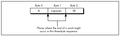
One detail remains to be attended to: setting the Carry flag for next time if the last byte was a non-separator. David does this in a bizarre and incredibly effective way: He presets the high bit of the count, and sets the high bit in the lookup table for those entries looked up by non-separators. When a non-separator’s lookup entry is added to the count, it will produce a carry, as desired. The high bit of the count is masked off before being added to the total count, so David is essentially using different parts of the count variables for different purposes (counting, and setting the Carry flag).
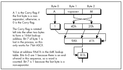
There are a number of other interesting details in David’s code, including the unrolling of the loop 64 times, so that 256 bytes in a row are processed without a single branch. Unfortunately, I lack the space to discuss Listing 16.5 any further. Perhaps that’s not so unfortunate, after all; I’d hate to deny you the pleasure of discovering the wonders of this rather remarkable code yourself. I will say one more thing, though. The cycle count for David’s inner loop is 6.5 cycles per byte processed, and the actual measured time for his routine, overhead and all, is 7.9 cycles/byte. The original C code clocked in at around 100 cycles/byte.
Enough said, I trust.
Enough Word Counting Already!
Before I finish up this chapter, I’d like to mention that Terje Mathisen’s WC word-counting program, which I’ve mentioned previously and which is available, with source, on Bix, is in the ballpark with David’s code for performance. What’s more, Terje’s program handles 8-bit ASCII, counts lines as well as words, and supports user-definable separator sets. It’s wonderful code, well worth a look; it also happens to be a great word-counting utility. By the way, Terje builds his 64K table on the fly, at program initialization; this allows for customized tables, shrinks the size of the EXE, and, according to Terje’s calculations, takes less time than loading the table off disk as part of the EXE.
So, has David written the fastest possible word-counting code? Well, maybe—but I have a letter from Terry Holmes, of San Rafael, California, that calculates the theoretical maximum performance of native 386 word-counting code at 5.5 cycles/byte, which would be significantly faster than David’s code. Terry, alas, didn’t bother to implement his design, but maybe I’ll take a shot at it someday. It’d be fun, for sure—but jeez, I’ve got real work to do!
Chapter 17 – The Game of Life
The Triumph of Algorithmic Optimization in a Cellular Automata Game
I’ve spent a lot of my life discussing assembly language optimization, which I consider to be an important and underappreciated topic. However, I’d like to take this opportunity to point out that there is much, much more to optimization than assembly language. Assembly is essential for absolute maximum performance, but it’s not the only ingredient; necessary but not sufficient, if you catch my drift—and not even necessary, if you’re looking for improved but not maximum performance. You’ve heard it a thousand times: Optimize your algorithm first. Devise new approaches. Or, as Knuth said, Premature optimization is the root of all evil.
This is, of course, old hat, stuff you know like the back of your hand. Or is it? As Jeff Duntemann pointed out to me the other day, performance programmers are made, not born. While I’m merrily gallivanting around in this book optimizing 486 pipelining and turning simple tasks into horribly complicated and terrifyingly fast state machines, many of you are still developing your basic optimization skills. I don’t want to shortchange those of you in the latter category, so in this chapter, we’ll discuss some high-level language optimizations that can be applied by mere mortals within a reasonable period of time. We’re going to examine a complete optimization process, from start to finish, and what we will find is that it’s possible to get a 50-times speed-up without using one byte of assembly! It’s all a matter of perspective—how you look at your code and data.
Conway’s Game
The program that we’re going to optimize is Conway’s famous Game of Life, long-ago favorite of the hackers at MIT’s AI Lab. If you’ve never seen it, let me assure you: Life is neat, and more than a little hypnotic. Fractals have been the hot graphics topic in recent years, but for eye-catching dazzle, Life is hard to beat.
Of course, eye-catching dazzle requires real-time performance—lots of pixels help too—and there’s the rub. When there are, say, 40,000 cells to process and display, a simple, straightforward implementation just doesn’t cut it, even on a 33 MHz 486. Happily, though, there are many, many ways to speed up Life, and they illustrate a variety of important optimization principles, as this chapter will show.
First, I’ll describe the ground rules of Life, implement a very straightforward version in C++, and then speed that version up by about eight times without using any drastically different approaches or any assembly. This may be a little tame for some of you, but be patient; for after that, we’ll haul out the big guns and move into the 30 to 40 times speed-up range. Then in the next chapter, I’ll show you how several programmers really floored it in taking me up on my second Optimization Challenge, which involved the Game of Life.
The Rules of the Game
The Game of Life is ridiculously simple. There is a cellmap, consisting of a rectangular matrix of cells, each of which may initially be either on or off. Each cell has eight neighbors: two horizontally, two vertically, and four diagonally. For each succeeding generation of cells, the game logic determines whether each cell will be on or off according to the following rules:
- If a cell is on and has either two or three neighbors that are on in the current generation, it stays on; otherwise, the cell turns off.
- If a cell is off and has exactly three “on” neighbors in the current generation, it turns on; otherwise, it stays off. That’s all the rules there are—but they give rise to an astonishing variety of forms, including patterns that spin, march across the screen, and explode.
It’s only a little more complicated to implement the Game of Life than it is to describe it. Listing 17.1, together with the display functions in Listing 17.2, is a C++ implementation of the Game of Life, and it’s very straightforward. A cellmap is an object that’s accessible through member functions to set, clear, and test cell states, and through a member function to calculate the next generation. Calculating the next generation involves nothing more than using the other member functions to set each cell to the appropriate state, given the number of neighboring on-cells and the cell’s current state. The only complication is that it’s necessary to place the next generation’s cells in another cellmap, and then copy the final result back to the original cellmap. This keeps us from corrupting the current generation’s cellmap before we’re done using it to calculate the next generation.
All in all, Listing 17.1 is a clean, compact, and elegant implementation of the Game of Life. Were it not that the code is as slow as molasses, we could stop right here.
LISTING 17.1 L17-1.CPP
/* C++ Game of Life implementation for any mode for which mode set
and draw pixel functions can be provided.
Tested with Borland C++ in the small model. */
#include <stdlib.h>
#include <stdio.h>
#include <iostream.h>
#include <conio.h>
#include <time.h>
#include <dos.h>
#include <bios.h>
#include <mem.h>
#define ON_COLOR 15 // on-cell pixel color
#define OFF_COLOR 0 // off-cell pixel color
#define MSG_LINE 10 // row for text messages
#define GENERATION_LINE 12 // row for generation # display
#define LIMIT_18_HZ 1 // set 1 for maximum frame rate = 18Hz
#define WRAP_EDGES 1 // set to 0 to disable wrapping around
// at cell map edges
class cellmap {
private:
unsigned char *cells;
unsigned int width;
unsigned int width_in_bytes;
unsigned int height;
unsigned int length_in_bytes;
public:
cellmap(unsigned int h, unsigned int v);
~cellmap(void);
void copy_cells(cellmap &sourcemap);
void set_cell(unsigned int x, unsigned int y);
void clear_cell(unsigned int x, unsigned int y);
int cell_state(int x, int y);
void next_generation(cellmap& dest_map);
};
extern void enter_display_mode(void);
extern void exit_display_mode(void);
extern void draw_pixel(unsigned int X, unsigned int Y,
unsigned int Color);
extern void show_text(int x, int y, char *text);
/* Controls the size of the cell map. Must be within the capabilities
of the display mode, and must be limited to leave room for text
display at right. */
unsigned int cellmap_width = 96;
unsigned int cellmap_height = 96;
/* Width & height in pixels of each cell as displayed on screen. */
unsigned int magnifier = 2;
void main()
{
unsigned int init_length, x, y, seed;
unsigned long generation = 0;
char gen_text[80];
long bios_time, start_bios_time;
cellmap current_map(cellmap_height, cellmap_width);
cellmap next_map(cellmap_height, cellmap_width);
// Get the seed; seed randomly if 0 entered
cout << "Seed (0 for random seed): ";
cin >> seed;
if (seed == 0) seed = (unsigned) time(NULL);
// Randomly initialize the initial cell map
cout << "Initializing...";
srand(seed);
init_length = (cellmap_height * cellmap_width) / 2;
do {
x = random(cellmap_width);
y = random(cellmap_height);
next_map.set_cell(x, y);
} while (--init_length);
current_map.copy_cells(next_map); // put init map in current_map
enter_display_mode();
// Keep recalculating and redisplaying generations until a key
// is pressed
show_text(0, MSG_LINE, "Generation: ");
start_bios_time = _bios_timeofday(_TIME_GETCLOCK, &bios_time);
do {
generation++;
sprintf(gen_text, "%10lu", generation);
show_text(1, GENERATION_LINE, gen_text);
// Recalculate and draw the next generation
current_map.next_generation(next_map);
// Make current_map current again
current_map.copy_cells(next_map);
#if LIMIT_18_HZ
// Limit to a maximum of 18.2 frames per second,for visibility
do {
_bios_timeofday(_TIME_GETCLOCK, &bios_time);
} while (start_bios_time == bios_time);
start_bios_time = bios_time;
#endif
} while (!kbhit());
getch(); // clear keypress
exit_display_mode();
cout << "Total generations: " << generation << "\nSeed: " <<
seed << "\n";
}
/* cellmap constructor. */
cellmap::cellmap(unsigned int h, unsigned int w)
{
width = w;
width_in_bytes = (w + 7) / 8;
height = h;
length_in_bytes = width_in_bytes * h;
cells = new unsigned char[length_in_bytes]; // cell storage
memset(cells, 0, length_in_bytes); // clear all cells, to start
}
/* cellmap destructor. */
cellmap::~cellmap(void)
{
delete[] cells;
}
/* Copies one cellmap's cells to another cellmap. Both cellmaps are
assumed to be the same size. */
void cellmap::copy_cells(cellmap &sourcemap)
{
memcpy(cells, sourcemap.cells, length_in_bytes);
}
/* Turns cell on. */
void cellmap::set_cell(unsigned int x, unsigned int y)
{
unsigned char *cell_ptr =
cells + (y * width_in_bytes) + (x / 8);
*(cell_ptr) |= 0x80 >> (x & 0x07);
}
/* Turns cell off. */
void cellmap::clear_cell(unsigned int x, unsigned int y)
{
unsigned char *cell_ptr =
cells + (y * width_in_bytes) + (x / 8);
*(cell_ptr) &= ~(0x80 >> (x & 0x07));
}
/* Returns cell state (1=on or 0=off), optionally wrapping at the
borders around to the opposite edge. */
int cellmap::cell_state(int x, int y)
{
unsigned char *cell_ptr;
#if WRAP_EDGES
while (x < 0) x += width; // wrap, if necessary
while (x >= width) x -= width;
while (y < 0) y += height;
while (y >= height) y -= height;
#else
if ((x < 0) || (x >= width) || (y < 0) || (y >= height))
return 0; // return 0 for off edges if no wrapping
#endif
cell_ptr = cells + (y * width_in_bytes) + (x / 8);
return (*cell_ptr & (0x80 >> (x & 0x07))) ? 1 : 0;
}
/* Calculates the next generation of a cellmap and stores it in
next_map. */
void cellmap::next_generation(cellmap& next_map)
{
unsigned int x, y, neighbor_count;
for (y=0; y<height; y++) {
for (x=0; x<width; x++) {
// Figure out how many neighbors this cell has
neighbor_count = cell_state(x-1, y-1) + cell_state(x, y-1) +
cell_state(x+1, y-1) + cell_state(x-1, y) +
cell_state(x+1, y) + cell_state(x-1, y+1) +
cell_state(x, y+1) + cell_state(x+1, y+1);
if (cell_state(x, y) == 1) {
// The cell is on; does it stay on?
if ((neighbor_count != 2) && (neighbor_count != 3)) {
next_map.clear_cell(x, y); // turn it off
draw_pixel(x, y, OFF_COLOR);
}
} else {
// The cell is off; does it turn on?
if (neighbor_count == 3) {
next_map.set_cell(x, y); // turn it on
draw_pixel(x, y, ON_COLOR);
}
}
}
}
}LISTING 17.2 L17-2.CPP
/* VGA mode 13h functions for Game of Life.
Tested with Borland C++. */
#include <stdio.h>
#include <conio.h>
#include <dos.h>
#define TEXT_X_OFFSET 27
#define SCREEN_WIDTH_IN_BYTES 320
/* Width & height in pixels of each cell. */
extern unsigned int magnifier;
/* Mode 13h draw pixel function. Pixels are of width & height
specified by magnifier. */
void draw_pixel(unsigned int x, unsigned int y, unsigned int color)
{
#define SCREEN_SEGMENT 0xA000
unsigned char far *screen_ptr;
int i, j;
FP_SEG(screen_ptr) = SCREEN_SEGMENT;
FP_OFF(screen_ptr) =
y * magnifier * SCREEN_WIDTH_IN_BYTES + x * magnifier;
for (i=0; i<magnifier; i++) {
for (j=0; j<magnifier; j++) {
*(screen_ptr+j) = color;
}
screen_ptr += SCREEN_WIDTH_IN_BYTES;
}
}
/* Mode 13h mode-set function. */
void enter_display_mode()
{
union REGS regset;
regset.x.ax = 0x0013;
int86(0x10, ®set, ®set);
}
/* Text mode mode-set function. */
void exit_display_mode()
{
union REGS regset;
regset.x.ax = 0x0003;
int86(0x10, ®set, ®set);
}
/* Text display function. Offsets text to non-graphics area of
screen. */
void show_text(int x, int y, char *text)
{
gotoxy(TEXT_X_OFFSET + x, y);
puts(text);
}Where Does the Time Go?
How slow is Listing 17.1? Table 17.1 shows that even on a 486,
Listing 17.1 does fewer than three 96x96 generations per second. (The
times in Table 17.1 are for 1,000 generations of a 96x96 cell map with
seed=1, LIMIT_18_HZ=0, WRAP_EDGES=1, and
magnifier=2, running on a 33 MHz 486.) Since my target is
18 generations per second with a 200x200 cellmap on a 20 MHz 386,
Listing 17.1 is too slow by a rather wide margin—75 times too slow, in
fact. You might say we have a little optimizing to do.
The first rule of optimization is: Only optimize where it matters.
Use a profiler, or risk making a fool of yourself. Consider Listings
17.1 and 17.2. Where do you think the potential for significant speed-up
lies? I’ll tell you one place where I thought there was considerable
potential—in draw_pixel(). As a programmer of high-speed
graphics, I figured any drawing function that was not only written in
C/C++ but also recalculated the target address from scratch for each
pixel would be among the first optimization targets. I also expected to
get major gains out of going to a Ping-Pong arrangement so that I didn’t
have to copy the new cellmap back to current_map after
calculating the next generation.
| Listing 17.1 | Listing 17.3 | Listing 17.4 | |
|---|---|---|---|
| Total execution time | 340 secs | 94 secs | 45 secs |
cell_state() |
275 | 21 | — |
next_generation() |
60 | 14 | 40 |
count_neighbors() |
— | 54 | — |
draw_pixel() |
2 | 2 | 2 |
set_cell() |
<1 | <1 | <1 |
clear_cell() |
<1 | <1 | <1 |
copy_cells() |
<1 | <1 | <1 |
I was wrong. Wrong, wrong, wrong. (But at least I was smart enough to
use a profiler before actually writing any new code.) Table 17.1 shows
where the time actually goes in Listings 17.1 and 17.2. As you can see,
the time taken by draw_pixel(), copy_cells(),
and everything other than calculating the next generation is
nothing more than noise. We could optimize these routines right down to
executing instantaneously, and you know what? It wouldn’t make
the slightest perceptible difference in how fast the program runs. Given
the present state of our Game of Life implementation, the only areas
worth looking at for possible optimizations are
cell_state() and next_generation().
draw_pixel()doesn’t much affect performance is that in Listing 17.1, we’re smart enough to redraw pixels only when their states change, rather than during every generation. Detecting and eliminating redundant operations is part of knowing the nature of your data, and is a potent optimization technique that will be extremely useful a little later in this chapter.
The Hazards and Advantages of Abstraction
How can we speed up cell_state() and
next_generation()? I’ll tell you how not to do it:
By writing those member functions in assembly. It’s tempting to say that
cell_state() is taking all the time, so we need to speed it
up with assembly, but what we really need to do is figure out
why cell_state() is taking all the time, then
address that aspect of the program directly.
Once you know where you need to optimize, the one word to keep in mind isn’t assembly, it’s…plastics. No, actually, it’s abstraction. Well-written C and especially C++ programs are highly abstract models. For example, Listing 17.1 essentially creates a new programming language in which cells are tangible things, with built-in manipulation instructions. Given the cellmap member functions, you don’t even need to know the cell storage format! This is a wonderful thing, in general; it saves programming time and bugs, and frees you to work on the application’s needs, rather than implementation details.
Having said that, let me hasten to add that algorithmic improvements
can make a big difference even when working at a purely abstract level.
For a large unordered data set, a high-level Quicksort will beat the
pants off the best-implemented insertion sort you can imagine. Still,
you can optimize your algorithm from here ’til doomsday, and if you have
a fast algorithm running on top of a highly abstract programming model,
you’ll almost certainly end up with a slow program. In Listing 17.1, the
abstraction that’s killing us is that of looking at the eight neighbors
with eight completely independent operations, requiring eight calls to
cell_state() and eight calculations of cell address and
cell mask. In fact, given the nature of cell storage, the eight
neighbors are in a fixed relationship to one another, and the addresses
and masks of all eight can generally be found very easily via hard-wired
offsets and shifts once the address and mask of any one is known.
There’s a kicker here, though, and that’s the counting of neighbors for cells at the edge of the cellmap. When cellmap wrapping is enabled (so that the cellmap becomes essentially a toroid, with each edge joined seamlessly to the opposite edge, as opposed to having a border of off-cells), neighbors that reside on the other edge of the cellmap can’t be accessed by the standard fixed offset, as shown in Figure 17.1. So, in general, we could improve performance by hard-wiring our neighbor-counting for the bit-per-cell cellmap format, but it seems we’d need a lot of conditional code to handle wrapping, and that would slow things back down again.
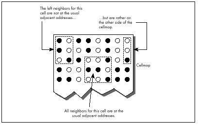
When a problem doesn’t lend itself well to optimization, make it a practice to see if you can change the problem definition to one that allows for greater efficiency. In this case, we’ll change the problem by putting padding bytes around the edge of the cellmap, and duplicating each edge of the cellmap in the padding bytes at the opposite side, as shown in Figure 17.2. That way, a hard-wired neighbor count will find exactly what it should—the opposite edge—without any special code at all.
But doesn’t that extra copying of the edges take time? Sure, but only
a little; we can build it into the cellmap copying function, and then
frankly we won’t even notice it. Avoiding tens or hundreds of thousands
of calls to cell_state(), on the other hand, will be
very noticeable. Listing 17.3 shows the alterations to Listing
17.1 required to implement a hard-wired neighbor-counting function. This
is a minor change, in truth, implemented in about half an hour and not
making the code significantly larger—but Listing 17.3 is 3.6 times
faster than Listing 17.1, as shown in Table 17.1. We’re up to about 10
generations per second on a 486; not where we want to be, but it is a
vast improvement.
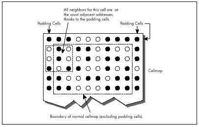
LISTING 17.3 L17-3.CPP
/* cellmap class definition, constructor, copy_cells(), set_cell(),
clear_cell(), cell_state(), count_neighbors(), and
next_generation() for fast, hard-wired neighbor count approach.
Otherwise, the same as Listing 17.1 */
class cellmap {
private:
unsigned char *cells;
unsigned int width;
unsigned int width_in_bytes;
unsigned int height;
unsigned int length_in_bytes;
public:
cellmap(unsigned int h, unsigned int v);
~cellmap(void);
void copy_cells(cellmap &sourcemap);
void set_cell(unsigned int x, unsigned int y);
void clear_cell(unsigned int x, unsigned int y);
int cell_state(int x, int y);
int count_neighbors(int x, int y);
void next_generation(cellmap& dest_map);
};
/* cellmap constructor. Pads around cell storage area with 1 extra
byte, used for handling edge wrapping. */
cellmap::cellmap(unsigned int h, unsigned int w)
{
width = w;
width_in_bytes = ((w + 7) / 8) + 2; // pad each side with
// 1 extra byte
height = h;
length_in_bytes = width_in_bytes * (h + 2); // pad top/bottom
// with 1 extra byte
cells = new unsigned char[length_in_bytes]; // cell storage
memset(cells, 0, length_in_bytes); // clear all cells, to start
}
/* Copies one cellmap's cells to another cellmap. If wrapping is
enabled, copies edge (wrap) bytes into opposite padding bytes in
source first, so that the padding bytes off each edge have the
same values as would be found by wrapping around to the opposite
edge. Both cellmaps are assumed to be the same size. */
void cellmap::copy_cells(cellmap &sourcemap)
{
unsigned char *cell_ptr;
int i;
#if WRAP_EDGES
// Copy left and right edges into padding bytes on right and left
cell_ptr = sourcemap.cells + width_in_bytes;
for (i=0; i<height; i++) {
*cell_ptr = *(cell_ptr + width_in_bytes - 2);
*(cell_ptr + width_in_bytes - 1) = *(cell_ptr + 1);
cell_ptr += width_in_bytes;
}
// Copy top and bottom edges into padding bytes on bottom and top
memcpy(sourcemap.cells, sourcemap.cells + length_in_bytes -
(width_in_bytes * 2), width_in_bytes);
memcpy(sourcemap.cells + length_in_bytes - width_in_bytes,
sourcemap.cells + width_in_bytes, width_in_bytes);
#endif
// Copy all cells to the destination
memcpy(cells, sourcemap.cells, length_in_bytes);
}
/* Turns cell on. x and y are offset by 1 byte down and to the right, to compensate for the
padding bytes around the cellmap. */
void cellmap::set_cell(unsigned int x, unsigned int y)
{
unsigned char *cell_ptr =
cells + ((y + 1) * width_in_bytes) + ((x / 8) + 1);
*(cell_ptr) |= 0x80 >> (x & 0x07);
}
/* Turns cell off. x and y are offset by 1 byte down and to the right,
to compensate for the padding bytes around the cell map. */
void cellmap::clear_cell(unsigned int x, unsigned int y)
{
unsigned char *cell_ptr =
cells + ((y + 1) * width_in_bytes) + ((x / 8) + 1);
*(cell_ptr) &= ~(0x80 >> (x & 0x07));
}
/* Returns cell state (1=on or 0=off). x and y are offset by 1 byte
down and to the right, to
compensate for the padding bytes around
the cell map. */
int cellmap::cell_state(int x, int y)
{
unsigned char *cell_ptr =
cells + ((y + 1) * width_in_bytes) + ((x / 8) + 1);
return (*cell_ptr & (0x80 >> (x & 0x07))) ? 1 : 0;
}
/* Counts the number of neighboring on-cells for specified cell. */
int cellmap::count_neighbors(int x, int y)
{
unsigned char *cell_ptr, mask;
unsigned int neighbor_count;
// Point to upper left neighbor
cell_ptr = cells + ((y * width_in_bytes) + ((x + 7) / 8));
mask = 0x80 >> ((x - 1) & 0x07);
// Count upper left neighbor
neighbor_count = (*cell_ptr & mask) ? 1 : 0;
// Count left neighbor
if ((*(cell_ptr + width_in_bytes) & mask)) neighbor_count++;
// Count lower left neighbor
if ((*(cell_ptr + (width_in_bytes * 2)) & mask)) neighbor_count++;
// Point to upper neighbor
if ((mask >>= 1) == 0) {
mask = 0x80;
cell_ptr++;
}
// Count upper neighbor
if ((*cell_ptr & mask)) neighbor_count++;
// Count lower neighbor
if ((*(cell_ptr + (width_in_bytes * 2)) & mask)) neighbor_count++;
// Point to upper right neighbor
if ((mask >>= 1) == 0) {
mask = 0x80;
cell_ptr++;
}
// Count upper right neighbor
if ((*cell_ptr & mask)) neighbor_count++;
// Count right neighbor
if ((*(cell_ptr + width_in_bytes) & mask)) neighbor_count++;
// Count lower right neighbor
if ((*(cell_ptr + (width_in_bytes * 2)) & mask)) neighbor_count++;
return neighbor_count;
}
/* Calculates the next generation of current_map and stores it in
next_map. */
void cellmap::next_generation(cellmap& next_map)
{
unsigned int x, y, neighbor_count;
for (y=0; y<height; y++) {
for (x=0; x<width; x++) {
neighbor_count = count_neighbors(x, y);
if (cell_state(x, y) == 1) {
if ((neighbor_count != 2) && (neighbor_count != 3)) {
next_map.clear_cell(x, y); // turn it off
draw_pixel(x, y, OFF_COLOR);
}
} else {
if (neighbor_count == 3) {
next_map.set_cell(x, y); // turn it on
draw_pixel(x, y, ON_COLOR);
}
}
}
}
}In Listing 17.3, note the padded cellmap edges, and the alteration of
the member functions to compensate for the padding. Also note that the
width now has to be a multiple of eight, to facilitate the process of
copying the edges to the opposite padding bytes. We have decreased the
generality of our Game of Life implementation in exchange for better
performance. That’s a very common trade-off, as common as trading memory
for performance. As a rule, the more general a program is, the slower it
is. A corollary is that often (not always, but often), the more heavily
optimized a program is, the more complex and the more difficult to
implement it is. You can often improve performance a good deal by
implementing only the level of generality you need, but at the same time
decreased generality makes it more difficult to change or port the
program at some later date. A Game of Life implementation, such as
Listing 17.1, that’s built on set_cell(),
clear_cell(), and get_cell() is completely
general; you can change the cell storage format simply by changing the
constructor and those three functions. Listing 17.3 is harder to change
because count_neighbors() would also have to be altered,
and it’s more complex than any of the other functions.
So, in Listing 17.3, we’ve gotten under the hood and changed the
cellmap format a little, and gotten impressive results. But now
count_neighbors() is hard-wired for optimized counting, and
it’s still taking up more than half the time. Maybe now it’s time to go
to assembly?
Not hardly.
Heavy-Duty C++ Optimization
Before we get to assembly, we still have to perform C++ optimization, then see if we can find an alternative approach that better fits the application. It would actually have made much more sense if we had looked for a new approach as our first optimization step, but I decided it would be better to cover straightforward C++ optimizations at this point, and the mind-bending stuff a little later. Right now, let’s look at some C++ optimizations; Listing 17.4 is a C++-optimized version of Listing 17.3.
LISTING 17.4 L17-4.CPP
/* next_generation(), implemented using fast, all-in-one hard-wired
neighbor count/update/draw function. Otherwise, the same as
Listing 17.3. */
/* Calculates the next generation of current_map and stores it in
next_map. */
void cellmap::next_generation(cellmap& next_map)
{
unsigned int x, y, neighbor_count;
unsigned int width_in_bytesX2 = width_in_bytes << 1;
unsigned char *cell_ptr, *current_cell_ptr, mask, current_mask;
unsigned char *base_cell_ptr, *row_cell_ptr, base_mask;
unsigned char *dest_cell_ptr = next_map.cells;
// Process all cells in the current cellmap
row_cell_ptr = cells; // point to upper left neighbor of
// first cell in cell map
for (y=0; y<height; y++) { // repeat for each row of cells
// Cell pointer and cell bit mask for first cell in row
base_cell_ptr = row_cell_ptr; // to access upper left neighbor
base_mask = 0x01; // of first cell in row
for (x=0; x<width; x++) { // repeat for each cell in row
// First, count neighbors
// Point to upper left neighbor of current cell
cell_ptr = base_cell_ptr; // pointer and bit mask for
mask = base_mask; // upper left neighbor
// Count upper left neighbor
neighbor_count = (*cell_ptr & mask) ? 1 : 0;
// Count left neighbor
if ((*(cell_ptr + width_in_bytes) & mask)) neighbor_count++;
// Count lower left neighbor
if ((*(cell_ptr + width_in_bytesX2) & mask))
neighbor_count++;
// Point to upper neighbor
if ((mask >>= 1) == 0) {
mask = 0x80;
cell_ptr++;
}
// Remember where to find the current cell
current_cell_ptr = cell_ptr + width_in_bytes;
current_mask = mask;
// Count upper neighbor
if ((*cell_ptr & mask)) neighbor_count++;
// Count lower neighbor
if ((*(cell_ptr + width_in_bytesX2) & mask))
neighbor_count++;
// Point to upper right neighbor
if ((mask >>= 1) == 0) {
mask = 0x80;
cell_ptr++;
}
// Count upper right neighbor
if ((*cell_ptr & mask)) neighbor_count++;
// Count right neighbor
if ((*(cell_ptr + width_in_bytes) & mask)) neighbor_count++;
// Count lower right neighbor
if ((*(cell_ptr + width_in_bytesX2) & mask))
neighbor_count++;
if (*current_cell_ptr & current_mask) {
if ((neighbor_count != 2) && (neighbor_count != 3)) {
*(dest_cell_ptr + (current_cell_ptr - cells)) &=
~current_mask; // turn off cell
draw_pixel(x, y, OFF_COLOR);
}
} else {
if (neighbor_count == 3) {
*(dest_cell_ptr + (current_cell_ptr - cells)) |=
current_mask; // turn on cell
draw_pixel(x, y, ON_COLOR);
}
}
// Advance to the next cell on row
if ((base_mask >>= 1) == 0) {
base_mask = 0x80;
base_cell_ptr++; // advance to the next cell byte
}
}
row_cell_ptr += width_in_bytes; // point to start of next row
}
}Listing 17.4 and Listing 17.3 are functionally the same; the only
difference lies in how next_generation() is implemented.
(Only next_generation() is shown in Listing 17.4; the
program is otherwise identical to Listing 17.3.) Listing 17.4 applies
the following optimizations to next_generation():
The neighbor-counting code is brought into
next_generation, eliminating many function calls and
from-scratch address/mask calculations; all multiplies are eliminated by
using pointers and addition; and all cells are accessed directly via
pointers and masks, eliminating all remaining function calls and
from-scratch address/mask calculations.
The net effect of these optimizations is that Listing 17.4 is more
than twice as fast as Listing 17.3; we’ve achieved the desired 18
generations per second, albeit only on a 486, and only at 96x96. (The
#define that enables code limiting the speed to 18 Hz,
which seemed ridiculous in Listing 17.1, is actually useful for keeping
the generations from iterating too quickly when Listing 17.4 is running
on a 486, especially with a small cellmap like 48x48.) We’ve sped things
up by about eight times so far; we need to increase our speed another
ten times to reach our goal of 200x200 at 18 generations per second on a
20 MHz 386.
It’s undoubtedly possible to improve the performance of Listing 17.4 further by fine-tuning the code, but no tremendous improvement is possible that way.
We’re still not ready for assembly, though; what we need is a new perspective that lends itself to vastly better performance in C++. The Life program in the next section is three to seven times faster than Listing 17.4—and it’s still in C++.
How is this possible? Here are some hints:
- After a few dozen generations, most of the cellmap consists of cells in the off state.
- There are many possible cellmap representations other than one bit-per-pixel.
- Cells change state relatively infrequently.
Bringing In the Right Brain
In the previous section, we saw how a C++ program could be sped up about eight times simply by rearranging the data and code in straightforward ways. Now we’re going to see how right-brain non-linear optimization can speed things up by another four times—and make the code simpler.
Now that’s Zen code optimization.
I have two objectives to achieve in the remainder of this chapter. First, I want to show that optimization consists of many levels, from assembly language up to conceptual design, and that assembly language kicks in pretty late in the optimization process. Second, I want to encourage you to saturate your brain with everything you know about any particular optimization problem, then make space for your right brain to solve the problem.
Re-Examining the Task
Earlier in this chapter, we looked at a straightforward Game of Life implementation, then increased performance considerably by making the implementation a little less abstract and a little less general. We made a small change to the cellmap format, adding padding bytes off the edges so that pointer arithmetic would always work, but the major optimizations were moving the critical code into a single loop and using pointers rather than member functions whenever possible. In other words, we took what we already knew and made it more efficient.
Now it’s time to re-examine the nature of this programming task from the ground up, looking for things that we don’t yet know. Let’s take a moment to review what the Game of Life consists of. The basic task is evolving a new generation, and that’s done by looking at the number of “on” neighbors a cell has and the cell’s own state. If a cell is on, and two or three neighbors are on, then the cell stays on; otherwise, an on-cell is turned off. If a cell is off and exactly three neighbors are on, then the cell is turned on; otherwise, an off-cell stays off. That’s all there is to it. As any fool can see, the trick is to arrange things so that we can count neighbors and check the cell state as quickly as possible. Large lookup tables, oddly encoded cellmaps, and lots of bit-twiddling assembly code spring to mind as possible approaches. Can’t you just feel your adrenaline start to pump?
What difference does that new perspective make? Let’s approach it this way. What does a typical cellmap look like? As it happens, after a few generations, the vast majority of cells are off. In fact, the vast majority of cells are not only off but are entirely surrounded by off-cells. Also, cells change state infrequently; in any given generation after the first few, most cells remain in the same state as in the previous generation.
Do you see where I’m heading? Do you hear a whisper of inspiration from your right brain? The original implementation stored cell states as 1-bits (on), or 0-bits (off). For each generation and for each cell, it counted the states of the eight neighbors, for an average of eight operations per cell per generation. Suppose, now, that on average 10 percent of cells change state from one generation to the next. (The actual percentage is even lower, but this will do for illustration.) Suppose also that we change the cell map format to store a byte rather than a bit for each cell, with the byte storing not only the cell state but also the count of neighboring on-cells for that cell. Figure 17.3 shows this format. Then, rather than counting neighbors each time, we could just look at the neighbor count in the cell and operate directly from that.
But what about the overhead needed to maintain the neighbor counts? Well, each time a cell changes state, eight operations would be needed to update the counts in the eight neighboring cells. But this happens only once every ten cells, on average—so the cost of this approach is only one-tenth that of the original approach!
Know your data.
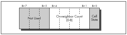
Acting on What We Know
Once we’ve changed the cellmap format to store neighbor counts as
well as states, with a byte for each cell, we can get another
performance boost by again examining what we know about our data. I said
earlier that most cells are off during any given generation. This means
that most cells have no neighbors that are on. Since the cell map
representation for an off-cell that has no neighbors is a zero byte, we
can skip over scads of unchanged cells at a pop simply by scanning for
non-zero bytes. This is much faster than explicitly testing cell states
and neighbor counts, and lends itself beautifully to assembly language
implementation as REPZ SCASB or (with a little cleverness)
REPZ SCASW. (Unfortunately, there’s no C library function
that can scan memory for the next byte that’s non-zero.)
Listing 17.5 is a Game of Life implementation that uses the neighbor-count cell map format and scans for non-zero bytes. On a 20 MHz 386, Listing 17.5 is about 4.5 times faster at calculating generations (that is, the generation engine is 4.5 times faster; I’m ignoring the time consumed by drawing and text display) than Listing 17.4, which is no slouch. On a 33 MHz 486, Listing 17.5 is about 3.5 times faster than Listing 17.4. This is true even though Listing 17.5 must be compiled using the large model. Imagine that—getting a four times speed-up while switching from the small model to the large model!
LISTING 17.5 L17-5.CPP
/* C++ Game of Life implementation for any mode for which mode set
and draw pixel functions can be provided. The cellmap stores the
neighbor count for each cell as well as the state of each cell;
this allows very fast next-state determination. Edges always wrap
in this implementation.
Tested with Borland C++. To run, link with Listing 17.2
in the large model. */
#include <stdlib.h>
#include <stdio.h>
#include <iostream.h>
#include <conio.h>
#include <time.h>
#include <dos.h>
#include <bios.h>
#include <mem.h>
#define ON_COLOR 15 // on-cell pixel color
#define OFF_COLOR 0 // off-cell pixel color
#define MSG_LINE 10 // row for text messages
#define GENERATION_LINE 12 // row for generation # display
#define LIMIT_18_HZ 0 // set 1 to to maximum frame rate = 18Hz
class cellmap {
private:
unsigned char *cells;
unsigned char *temp_cells;
unsigned int width;
unsigned int height;
unsigned int length_in_bytes;
public:
cellmap(unsigned int h, unsigned int v);
~cellmap(void);
void set_cell(unsigned int x, unsigned int y);
void clear_cell(unsigned int x, unsigned int y);
int cell_state(int x, int y);
int count_neighbors(int x, int y);
void next_generation(void);
void init(void);
};
extern void enter_display_mode(void);
extern void exit_display_mode(void);
extern void draw_pixel(unsigned int X, unsigned int Y,
unsigned int Color);
extern void show_text(int x, int y, char *text);
/* Controls the size of the cell map. Must be within the capabilities
of the display mode, and must be limited to leave room for text
display at right. */
unsigned int cellmap_width = 96;
unsigned int cellmap_height = 96;
/* Width & height in pixels of each cell. */
unsigned int magnifier = 2;
/* Randomizing seed */
unsigned int seed;
void main()
{
unsigned long generation = 0;
char gen_text[80];
long bios_time, start_bios_time;
cellmap current_map(cellmap_height, cellmap_width);
current_map.init(); // randomly initialize cell map
enter_display_mode();
// Keep recalculating and redisplaying generations until any key
// is pressed
show_text(0, MSG_LINE, "Generation: ");
start_bios_time = _bios_timeofday(_TIME_GETCLOCK, &bios_time);
do {
generation++;
sprintf(gen_text, "%10lu", generation);
show_text(1, GENERATION_LINE, gen_text);
// Recalculate and draw the next generation
current_map.next_generation();
#if LIMIT_18_HZ
// Limit to a maximum of 18.2 frames per second, for visibility
do {
_bios_timeofday(_TIME_GETCLOCK, &bios_time);
} while (start_bios_time == bios_time);
start_bios_time = bios_time;
#endif
} while (!kbhit());
getch(); // clear keypress
exit_display_mode();
cout << "Total generations: " << generation << "\nSeed: " <<
seed << "\n";
}
/* cellmap constructor. */
cellmap::cellmap(unsigned int h, unsigned int w)
{
width = w;
height = h;
length_in_bytes = w * h;
cells = new unsigned char[length_in_bytes]; // cell storage
temp_cells = new unsigned char[length_in_bytes]; // temp cell storage
if ( (cells == NULL) || (temp_cells == NULL) ) {
printf("Out of memory\n");
exit(1);
}
memset(cells, 0, length_in_bytes); // clear all cells, to start
}
/* cellmap destructor. */
cellmap::~cellmap(void)
{
delete[] cells;
delete[] temp_cells;
}
/* Turns an off-cell on, incrementing the on-neighbor count for the
eight neighboring cells. */
void cellmap::set_cell(unsigned int x, unsigned int y)
{
unsigned int w = width, h = height;
int xoleft, xoright, yoabove, yobelow;
unsigned char *cell_ptr = cells + (y * w) + x;
// Calculate the offsets to the eight neighboring cells,
// accounting for wrapping around at the edges of the cell map
if (x == 0)
xoleft = w - 1;
else
xoleft = -1;
if (y == 0)
yoabove = length_in_bytes - w;
else
yoabove = -w;
if (x == (w - 1))
xoright = -(w - 1);
else
xoright = 1;
if (y == (h - 1))
yobelow = -(length_in_bytes - w);
else
yobelow = w;
*(cell_ptr) |= 0x01;
*(cell_ptr + yoabove + xoleft) += 2;
*(cell_ptr + yoabove) += 2;
*(cell_ptr + yoabove + xoright) += 2;
*(cell_ptr + xoleft) += 2;
*(cell_ptr + xoright) += 2;
*(cell_ptr + yobelow + xoleft) += 2;
*(cell_ptr + yobelow) += 2;
*(cell_ptr + yobelow + xoright) += 2;
}
/* Turns an on-cell off, decrementing the on-neighbor count for the
eight neighboring cells. */
void cellmap::clear_cell(unsigned int x, unsigned int y)
{
unsigned int w = width, h = height;
int xoleft, xoright, yoabove, yobelow;
unsigned char *cell_ptr = cells + (y * w) + x;
// Calculate the offsets to the eight neighboring cells,
// accounting for wrapping around at the edges of the cell map
if (x == 0)
xoleft = w - 1;
else
xoleft = -1;
if (y == 0)
yoabove = length_in_bytes - w;
else
yoabove = -w;
if (x == (w - 1))
xoright = -(w - 1);
else
xoright = 1;
if (y == (h - 1))
yobelow = -(length_in_bytes - w);
else
yobelow = w;
*(cell_ptr) &= ~0x01;
*(cell_ptr + yoabove + xoleft) -= 2;
*(cell_ptr + yoabove ) -= 2;
*(cell_ptr + yoabove + xoright) -= 2;
*(cell_ptr + xoleft) -= 2;
*(cell_ptr + xoright) -= 2;
*(cell_ptr + yobelow + xoleft) -= 2;
*(cell_ptr + yobelow) -= 2;
*(cell_ptr + yobelow + xoright) -= 2;
}
/* Returns cell state (1=on or 0=off). */
int cellmap::cell_state(int x, int y)
{
unsigned char *cell_ptr;
cell_ptr = cells + (y * width) + x;
return *cell_ptr & 0x01;
}
/* Calculates and displays the next generation of current_map */
void cellmap::next_generation()
{
unsigned int x, y, count;
unsigned int h = height, w = width;
unsigned char *cell_ptr, *row_cell_ptr;
// Copy to temp map, so we can have an unaltered version from
// which to work
memcpy(temp_cells, cells, length_in_bytes);
// Process all cells in the current cell map
cell_ptr = temp_cells; // first cell in cell map
for (y=0; y<h; y++) { // repeat for each row of cells
// Process all cells in the current row of the cell map
x = 0;
do { // repeat for each cell in row
// Zip quickly through as many off-cells with no
// neighbors as possible
while (*cell_ptr == 0) {
cell_ptr++; // advance to the next cell
if (++x >= w) goto RowDone;
}
// Found a cell that's either on or has on-neighbors,
// so see if its state needs to be changed
count = *cell_ptr >> 1; // # of neighboring on-cells
if (*cell_ptr & 0x01) {
// Cell is on; turn it off if it doesn't have
// 2 or 3 neighbors
if ((count != 2) && (count != 3)) {
clear_cell(x, y);
draw_pixel(x, y, OFF_COLOR);
}
} else {
// Cell is off; turn it on if it has exactly 3 neighbors
if (count == 3) {
set_cell(x, y);
draw_pixel(x, y, ON_COLOR);
}
}
// Advance to the next cell
cell_ptr++; // advance to the next cell byte
} while (++x < w);
RowDone:
}
}
/* Randomly initializes the cellmap to about 50% on-pixels. */
void cellmap::init()
{
unsigned int x, y, init_length;
// Get the seed; seed randomly if 0 entered
cout << "Seed (0 for random seed): ";
cin >> seed;
if (seed == 0) seed = (unsigned) time(NULL);
// Randomly initialize the initial cell map to 50% on-pixels
// (actually generally fewer, because some coordinates will be
// randomly selected more than once)
cout << "Initializing...";
srand(seed);
init_length = (height * width) / 2;
do {
x = random(width);
y = random(height);
if (cell_state(x, y) == 0) {
set_cell(x, y);
}
} while (--init_length);
}The large model is actually not necessary for the 96x96 cellmap in Listing 17.5. However, I was actually more interested in seeing a fast 200x200 cellmap, and two 200x200 cellmaps can’t fit in a single segment. (This can easily be worked around in assembly language for cellmaps up to a segment in size; beyond that size, cellmap scanning becomes pretty complex, although it can still be efficiently implemented with some clever programming.)
Anyway, using the large model helps illustrate that it’s the data representation and the data processing approach you choose that matter most. Optimization details like memory models and segments and in-line functions and assembly language are important but secondary. Let your mind roam creatively before you start coding. Otherwise, you may find you’re writing well-tuned slow code, which is by no means the same thing as fast code.
Take a close look at Listing 17.5. You will see that it’s quite a bit
simpler than Listing 17.4. To some extent, that’s because I decided to
hard-wire the program to wrap around from one edge of the cellmap to the
other (it’s much more interesting that way), but the main reason is that
it’s a lot easier to work with the neighbor-count model. There’s no
complex mask and pointer management, and the only thing that
really needs to be optimized is scanning for zero bytes. (And,
in fact, I haven’t optimized even that because it’s done in a C++ loop;
it should really be REPZ SCASB.)
In truth, none of the code in Listing 17.5 is particularly well-optimized, and, as I noted, the program must be compiled with the large model for large cellmaps. Also, of course, the entire program is still in C++; note well that there’s not a whit of assembly here.
No doubt we could get another two to five times improvement with good assembly code—but that’s dwarfed by a 30-times improvement, so optimization at a conceptual level must come first.
The Challenge That Ate My Life
The most recent optimization challenge I laid my community of readers was to write the fastest possible Game of Life generation engine. By “engine” I meant that I didn’t care about time spent in input or output, only time consumed by the call to next-generation. The time spent updating the cellmap was what I wanted people to concentrate on.
Here are the rules I laid down for the challenge:
- Readers could modify any code in Listing 17.5, except the main loop, as well as change the cell map representation any way they liked. However, the code had to produce exactly the same output as Listing 17.5 under all circumstances in order to be eligible to win.
- Engine code had to be less than 400 lines long in total, excluding the video-related code shown in Listing 17.2.
- Submissions had to compile/assemble with Borland C++ (in either C++ or C mode, as desired) and/or TASM.
- All submissions had to handle cellmaps at least 200x200 in size.
- Assembly language could of course be used to speed up any part of the program. C rather than C++ was legal as well, so long as entered implementations produced the same results as Listing 17.5 and 17.2 together and were less than 400 lines long.
- All entries would be timed on the same 33 MHz 486 with a 256K external cache.
That was the challenge I put to the readers. Little did I realize the challenge it would lay on me: Entries poured in from the four corners of the globe. Some were plain, some were brilliant, some were, well, berserk. Many didn’t even work. But all had to be gone through, examined for adherence to the rules, read, compiled, linked, run, and judged. I learned a lot—about a lot of things, not the least of which was the process (or maybe the wisdom) of laying down challenges to readers.
Who won? What did I learn? To find out, read on.
Chapter 18 – It’s a plain Wonderful Life
Optimization beyond the Pale
When I was in high school, my gym teacher had us run a race around the soccer field, or rather, around a course marked with cones that roughly outlined the shape of the field. I quickly settled into second place behind Dwight Chamberlin. We cruised around the field, and when we came to the far corner, Dwight cut across the corner, inside a cone placed awkwardly far out from the others. I followed, and everyone else cut inside the cone too—except the pear-shaped kid bringing up the rear, who plodded his way around every single cone on his way to finishing about half a lap behind. When the laggard finally crossed the finish line, the coach named him the winner, to my considerable irritation. After all, the object was to see who could run the fastest, wasn’t it?
Actually, it wasn’t. The object was to see who could run the fastest according to the limitations placed upon the contest. This is a crucial distinction, although usually taken for granted. Would it have been legitimate if I had cut across the middle of the field? If I had ridden a bike? If I had broken the world record for the 100 meters by dropping 100 meters from a plane? Competition has meaning only within a carefully circumscribed arena.
Why am I telling you this? First, because it is a useful lesson for programming.
Breaking the Rules
The other reason for the anecdote has to do with the way my second Optimization Challenge worked itself out. If you’ll recall from the last chapter, the challenge I made to the readers of PC TECHNIQUES was to devise the fastest possible version of the Game of Life cellular automata simulation game. I gave an example, laid out the rules, and stood aside. Good thing, too. Apres moi, le deluge….
And when the dust had settled, I was left with the uneasy realization that every submitted entry broke the rules. Every single entry. The rules clearly stated that submitted code must produce exactly the same output as my example implementation under all circumstances in order to be eligible to win. I do not think that there can be any question about what “exactly the same output” means. It means the same pixels, in the same colors, at the same places on the screen at the same points in all the Life simulations that the original code was capable of running. Period. And not one of the entries met that standard. Some submitted listings were more than 400 lines long. Some didn’t display the generation number at the right side of the screen, didn’t draw the same pixel colors, or didn’t bother with magnification. Some had bugs. Some didn’t support all possible cellmap widths and heights up to 200x200, requiring widths and heights that were specific multiples of a number of cells that lent itself to a particular implementation.
This last mission is, in a way, a brilliant approach, as evidenced by the fact that it yielded the two fastest submissions, but it is not within the rules of the contest. Some of the rule-breaking was major, some very minor, and some had nothing to do with the Life engine itself, but the rules were clear; where was I to draw the line if not with exact compliance? And I was fully prepared to draw that line rigorously, disqualifying some mind-bending submissions in order to let lesser but fully compliant entries win—until I realized that there were no fully compliant entries.
Given which, I heaved a sigh of relief, threw away the rules, and picked a winner in the true spirit of the contest: raw speed. Two winners, in fact: Peter Klerings, a programmer for Turck GmbH in Munich, Germany, whose entry just plain runs like a bat out of hell, and David Stafford (who was also the winner of my first Optimization Challenge), of Borland International, whose entry is slightly slower mainly because he didn’t optimize the drawing part of the program, in full accordance with the contest rules, which specifically excluded drawing time from consideration. Unfortunately, Peter’s generation code and drawing code are so tightly intertwined that it is impossible to separate them, and hence not really possible to figure out whose generation engine is faster. Anyway, at 180 to 200 generations per second, including drawing time, for 200x200 cellmaps (and in the neighborhood of 1000 gps for 96x96 cellmaps, the size of my original implementation), they’re the fastest submissions I received. They’re both more than an order of magnitude faster than my final optimized C++ Life implementation shown in Chapter 17, and more than 300 times faster than my original, perfectly functional Life implementation. Not 300 percent—300 times. Cell generations scud across the screen like clouds, and walkers shoot out like bullets. Each is a worthy winner, and I feel confident that the true objective of the challenge has been met: pure, breathtaking speed.
Notwithstanding, mea culpa. The next time I lay a challenge, I will define the rules with scrupulous care. Even so, this was much more than just another cycle-counting contest. We’re fortunate enough to be privy to a startling demonstration of the power of the best optimizer anyone has yet devised—you. (That’s the general “you”; I realize that the specific “you” may or may not be quite up to the optimizing level of the specific “David Stafford” or “Peter Klerings.”)
Onward to the code.
Table-Driven Magic
David Stafford won my first Optimization Challenge by means of a huge look-up table and an incredible state machine driven by that table. The table didn’t cause David’s entry to exceed the line limit because David’s submission included code to generate the table on the fly as part of the build process. David has done himself one better this time with his QLIFE program; not only does his build process generate a 64K table, but it also generates virtually all his code, consisting of 17,000-plus lines of assembly language spanning another 64K. What David has done is write the equivalent of a bitblt compiler for the Game of Life; one might in fact call it a Life compiler. What David’s code generates is still a general-purpose program; it takes arbitrary seed values, and can run for an arbitrary number of generations, so it’s not as if David simply hardwired the instructions to draw each successive screen. However, it’s a general-purpose program that is exquisitely tailored to the task it needs to perform.
All the pieces of QLIFE are shown in Listings 18.1 through 18.5, as follows: Listing 18.1 is BUILD.BAT, the batch file used to build QLIFE; Listing 18.2 is LCOMP.C, the program used to generate the assembler code and data file QLIFE.ASM; Listing 18.3 is MAIN.C, the main program for QLIFE; Listing 18.4 is VIDEO.C, the video-related functions, and Listing 18.5 is LIFE.H, the header file. The following sidebar contains David’s build instructions, exactly as he wrote them. I certainly won’t have room to discuss all the marvelous intricacies of David’s code; I suggest you look over these listings until you understand them thoroughly (it took me a day to pick them apart) because there’s a lot of neat stuff in there, and it’s an approach to performance programming that operates at a more efficient, tightly integrated level than you may ever see again. One hint: It helps a lot to build and run LCOMP.C, redirect its output to QLIFE.ASM, and look at the assembly code in that file. This code is the entirety of David’s generation engine, and it’s almost impossible to visualize its operation without actually seeing it.
How To Build Qlife
QLIFE is written for Borland C++, but it shouldn’t be too difficult to convert it to work with Microsoft C++. To build QLIFE, run the BUILD.BAT batch file with the size of the life grid on the command line (see below). The command-line options are:
WIDTH 32 Sets the width of the life grid to 96 cells (divided by 3). HEIGHT 96 Sets the height of the life grid to 96 cells. NOCOUNTER Turns off the generation counter (optional). NODRAW Turns off drawing of the cell map (optional). GEN 1000 Calculates 1,000 generations (optional). These must be in uppercase. For example, the minimum you really need is “WIDTH 40 HEIGHT 120.” I used “WIDTH 46 HEIGHT 138 NOCOUNTER NODRAW GEN 7000” during testing.
If you have selected the GEN option, you will have to press a key to exit QLIFE when it is finished. This is so I could visually compare the result of N generations under QLIFE with N generations under Abrash’s original life program. You should be aware that the program from the listing contains a small bug, which may make it appear that they do not generate identical results. The original program does not display a cell until it changes, so if a cell is alive on the first generation and never dies, then it will never be displayed. This bug is not present in QLIFE.
You should have no trouble running QLIFE with cell grids up to 210x200.
You must have a VGA and at least a 386 to run QLIFE. The 386 features that it uses are not integral to the algorithm (they’re a convenience for the code), so feel free to modify QLIFE to run on earlier CPUs if you wish. QLIFE works best if you have a large CPU cache (256K is recommended).
—David Stafford
LISTING 18.1 BUILD.BAT
bcc -v -D%1=%2;%2=%3;%3=%4;%4=%5;%5=%6;%6=%7;%7=%8;%8 lcomp.c
lcomp > qlife.asm
tasmx /mx /kh30000 qlife
bcc -v -D%1=%2;%2=%3;%3=%4;%4=%5;%5=%6;%6=%7;%7=%8;%8 qlife.obj main.c video.cLISTING 18.2 LCOMP.C
// LCOMP.C
//
// Life compiler, ver 1.3
//
// David Stafford
//
#include <stdio.h>
#include <stdlib.h>
#include "life.h"
#define LIST_LIMIT (46 * 138) // when we need to use es:
int Old, New, Edge, Label;
char Buf[ 20 ];
void Next1( void )
{
char *Seg = "";
if( WIDTH * HEIGHT > LIST_LIMIT ) Seg = "es:";
printf( "mov bp,%s[si]\n", Seg );
printf( "add si,2\n" );
printf( "mov dh,[bp+1]\n" );
printf( "and dh,0FEh\n" );
printf( "jmp dx\n" );
}
void Next2( void )
{
printf( "mov bp,es:[si]\n" );
printf( "add si,2\n" );
printf( "mov dh,[bp+1]\n" );
printf( "or dh,1\n" );
printf( "jmp dx\n" );
}
void BuildMaps( void )
{
unsigned short i, j, Size, x = 0, y, N1, N2, N3, C1, C2, C3;
printf( "_DATA segment 'DATA'\nalign 2\n" );
printf( "public _CellMap\n" );
printf( "_CellMap label word\n" );
for( j = 0; j < HEIGHT; j++ )
{
for( i = 0; i < WIDTH; i++ )
{
if( i == 0 || i == WIDTH-1 || j == 0 || j == HEIGHT-1 )
{
printf( "dw 8000h\n" );
}
else
{
printf( "dw 0\n" );
}
}
}
printf( "ChangeCell dw 0\n" );
printf( "_RowColMap label word\n" );
for( j = 0; j < HEIGHT; j++ )
{
for( i = 0; i < WIDTH; i++ )
{
printf( "dw 0%02x%02xh\n", j, i * 3 );
}
}
if( WIDTH * HEIGHT > LIST_LIMIT )
{
printf( "Change1 dw offset _CHANGE:_ChangeList1\n" );
printf( "Change2 dw offset _CHANGE:_ChangeList2\n" );
printf( "ends\n\n" );
printf( "_CHANGE segment para public 'FAR_DATA'\n" );
}
else
{
printf( "Change1 dw offset DGROUP:_ChangeList1\n" );
printf( "Change2 dw offset DGROUP:_ChangeList2\n" );
}
Size = WIDTH * HEIGHT + 1;
printf( "public _ChangeList1\n_ChangeList1 label word\n" );
printf( "dw %d dup (offset DGROUP:ChangeCell)\n", Size );
printf( "public _ChangeList2\n_ChangeList2 label word\n" );
printf( "dw %d dup (offset DGROUP:ChangeCell)\n", Size );
printf( "ends\n\n" );
printf( "_LDMAP segment para public 'FAR_DATA'\n" );
do
{
// Current cell states
C1 = (x & 0x0800) >> 11;
C2 = (x & 0x0400) >> 10;
C3 = (x & 0x0200) >> 9;
// Neighbor counts
N1 = (x & 0x01C0) >> 6;
N2 = (x & 0x0038) >> 3;
N3 = (x & 0x0007);
y = x & 0x8FFF; // Preserve all but the next generation states
if( C1 && ((N1 + C2 == 2) || (N1 + C2 == 3)) )
{
y |= 0x4000;
}
if( !C1 && (N1 + C2 == 3) )
{
y |= 0x4000;
}
if( C2 && ((N2 + C1 + C3 == 2) || (N2 + C1 + C3 == 3)) )
{
y |= 0x2000;
}
if( !C2 && (N2 + C1 + C3 == 3) )
{
y |= 0x2000;
}
if( C3 && ((N3 + C2 == 2) || (N3 + C2 == 3)) )
{
y |= 0x1000;
}
if( !C3 && (N3 + C2 == 3) )
{
y |= 0x1000;
}
printf( "db 0%02xh\n", y >> 8 );
}
while( ++x != 0 );
printf( "ends\n\n" );
}
void GetUpAndDown( void )
{
printf( "mov ax,[bp+_RowColMap-_CellMap]\n" );
printf( "or ah,ah\n" );
printf( "mov dx,%d\n", DOWN );
printf( "mov cx,%d\n", WRAPUP );
printf( "jz short D%d\n", Label );
printf( "cmp ah,%d\n", HEIGHT - 1 );
printf( "mov cx,%d\n", UP );
printf( "jb short D%d\n", Label );
printf( "mov dx,%d\n", WRAPDOWN );
printf( "D%d:\n", Label );
}
void FirstPass( void )
{
char *Op;
unsigned short UpDown = 0;
printf( "org 0%02x00h\n", (Edge << 7) + (New << 4) + (Old << 1) );
// reset cell
printf( "xor byte ptr [bp+1],0%02xh\n", (New ^ Old) << 1 );
// get the screen address and update the display
#ifndef NODRAW
printf( "mov al,160\n" );
printf( "mov bx,[bp+_RowColMap-_CellMap]\n" );
printf( "mul bh\n" );
printf( "add ax,ax\n" );
printf( "mov bh,0\n" );
printf( "add bx,ax\n" ); // bx = screen offset
if( ((New ^ Old) & 6) == 6 )
{
printf( "mov word ptr fs:[bx],0%02x%02xh\n",
(New & 2) ? 15 : 0,
(New & 4) ? 15 : 0 );
if( (New ^ Old) & 1 )
{
printf( "mov byte ptr fs:[bx+2],%s\n",
(New & 1) ? "15" : "dl" );
}
}
else
{
if( ((New ^ Old) & 3) == 3 )
{
printf( "mov word ptr fs:[bx+1],0%02x%02xh\n",
(New & 1) ? 15 : 0,
(New & 2) ? 15 : 0 );
}
else
{
if( (New ^ Old) & 2 )
{
printf( "mov byte ptr fs:[bx+1],%s\n",
(New & 2) ? "15" : "dl" );
}
if( (New ^ Old) & 1 )
{
printf( "mov byte ptr fs:[bx+2],%s\n",
(New & 1) ? "15" : "dl" );
}
}
if( (New ^ Old) & 4 )
{
printf( "mov byte ptr fs:[bx],%s\n",
(New & 4) ? "15" : "dl" );
}
}
#endif
if( (New ^ Old) & 4 ) UpDown += (New & 4) ? 0x48 : -0x48;
if( (New ^ Old) & 2 ) UpDown += (New & 2) ? 0x49 : -0x49;
if( (New ^ Old) & 1 ) UpDown += (New & 1) ? 0x09 : -0x09;
if( Edge )
{
GetUpAndDown(); // ah = row, al = col, cx = up, dx = down
if( (New ^ Old) & 4 )
{
printf( "mov di,%d\n", WRAPLEFT ); // di = left
printf( "cmp al,0\n" );
printf( "je short L%d\n", Label );
printf( "mov di,%d\n", LEFT );
printf( "L%d:\n", Label );
if( New & 4 ) Op = "inc";
else Op = "dec";
printf( "%s word ptr [bp+di]\n", Op );
printf( "add di,cx\n" );
printf( "%s word ptr [bp+di]\n", Op );
printf( "sub di,cx\n" );
printf( "add di,dx\n" );
printf( "%s word ptr [bp+di]\n", Op );
}
if( (New ^ Old) & 1 )
{
printf( "mov di,%d\n", WRAPRIGHT ); // di = right
printf( "cmp al,%d\n", (WIDTH - 1) * 3 );
printf( "je short R%d\n", Label );
printf( "mov di,%d\n", RIGHT );
printf( "R%d:\n", Label );
if( New & 1 ) Op = "add";
else Op = "sub";
printf( "%s word ptr [bp+di],40h\n", Op );
printf( "add di,cx\n" );
printf( "%s word ptr [bp+di],40h\n", Op );
printf( "sub di,cx\n" );
printf( "add di,dx\n" );
printf( "%s word ptr [bp+di],40h\n", Op );
}
printf( "mov di,cx\n" );
printf( "add word ptr [bp+di],%d\n", UpDown );
printf( "mov di,dx\n" );
printf( "add word ptr [bp+di],%d\n", UpDown );
printf( "mov dl,0\n" );
}
else
{
if( (New ^ Old) & 4 )
{
if( New & 4 ) Op = "inc";
else Op = "dec";
printf( "%s byte ptr [bp+%d]\n", Op, LEFT );
printf( "%s byte ptr [bp+%d]\n", Op, UPPERLEFT );
printf( "%s byte ptr [bp+%d]\n", Op, LOWERLEFT );
}
if( (New ^ Old) & 1 )
{
if( New & 1 ) Op = "add";
else Op = "sub";
printf( "%s word ptr [bp+%d],40h\n", Op, RIGHT );
printf( "%s word ptr [bp+%d],40h\n", Op, UPPERRIGHT );
printf( "%s word ptr [bp+%d],40h\n", Op, LOWERRIGHT );
}
if( abs( UpDown ) > 1 )
{
printf( "add word ptr [bp+%d],%d\n", UP, UpDown );
printf( "add word ptr [bp+%d],%d\n", DOWN, UpDown );
}
else
{
if( UpDown == 1 ) Op = "inc";
else Op = "dec";
printf( "%s byte ptr [bp+%d]\n", Op, UP );
printf( "%s byte ptr [bp+%d]\n", Op, DOWN );
}
}
Next1();
}
void Test( char *Offset, char *Str )
{
printf( "mov bx,[bp+%s]\n", Offset );
printf( "cmp bh,[bx]\n" );
printf( "jnz short FIX_%s%d\n", Str, Label );
printf( "%s%d:\n", Str, Label );
}
void Fix( char *Offset, char *Str, int JumpBack )
{
printf( "FIX_%s%d:\n", Str, Label );
printf( "mov bh,[bx]\n" );
printf( "mov [bp+%s],bx\n", Offset );
if( *Offset != '0' ) printf( "lea ax,[bp+%s]\n", Offset );
else printf( "mov ax,bp\n" );
printf( "stosw\n" );
if( JumpBack ) printf( "jmp short %s%d\n", Str, Label );
}
void SecondPass( void )
{
printf( "org 0%02x00h\n",
(Edge << 7) + (New << 4) + (Old << 1) + 1 );
if( Edge )
{
// finished with second pass
if( New == 7 && Old == 0 )
{
printf( "cmp bp,offset DGROUP:ChangeCell\n" );
printf( "jne short NotEnd\n" );
printf( "mov word ptr es:[di],offset DGROUP:ChangeCell\n" );
printf( "pop di si bp ds\n" );
printf( "mov ChangeCell,0\n" );
printf( "retf\n" );
printf( "NotEnd:\n" );
}
GetUpAndDown(); // ah = row, al = col, cx = up, dx = down
printf( "push si\n" );
printf( "mov si,%d\n", WRAPLEFT ); // si = left
printf( "cmp al,0\n" );
printf( "je short L%d\n", Label );
printf( "mov si,%d\n", LEFT );
printf( "L%d:\n", Label );
Test( "si", "LEFT" );
printf( "add si,cx\n" );
Test( "si", "UPPERLEFT" );
printf( "sub si,cx\n" );
printf( "add si,dx\n" );
Test( "si", "LOWERLEFT" );
printf( "mov si,cx\n" );
Test( "si", "UP" );
printf( "mov si,dx\n" );
Test( "si", "DOWN" );
printf( "cmp byte ptr [bp+_RowColMap-_CellMap],%d\n",
(WIDTH - 1) * 3 );
printf( "mov si,%d\n", WRAPRIGHT ); // si = right
printf( "je short R%d\n", Label );
printf( "mov si,%d\n", RIGHT );
printf( "R%d:\n", Label );
Test( "si", "RIGHT" );
printf( "add si,cx\n" );
Test( "si", "UPPERRIGHT" );
printf( "sub si,cx\n" );
printf( "add si,dx\n" );
Test( "si", "LOWERRIGHT" );
}
else
{
Test( itoa( LEFT, Buf, 10 ), "LEFT" );
Test( itoa( UPPERLEFT, Buf, 10 ), "UPPERLEFT" );
Test( itoa( LOWERLEFT, Buf, 10 ), "LOWERLEFT" );
Test( itoa( UP, Buf, 10 ), "UP" );
Test( itoa( DOWN, Buf, 10 ), "DOWN" );
Test( itoa( RIGHT, Buf, 10 ), "RIGHT" );
Test( itoa( UPPERRIGHT, Buf, 10 ), "UPPERRIGHT" );
Test( itoa( LOWERRIGHT, Buf, 10 ), "LOWERRIGHT" );
}
if( New == Old ) Test( "0", "CENTER" );
if( Edge ) printf( "pop si\n" "mov dl,0\n" );
Next2();
if( Edge )
{
Fix( "si", "LEFT", 1 );
Fix( "si", "UPPERLEFT", 1 );
Fix( "si", "LOWERLEFT", 1 );
Fix( "si", "UP", 1 );
Fix( "si", "DOWN", 1 );
Fix( "si", "RIGHT", 1 );
Fix( "si", "UPPERRIGHT", 1 );
Fix( "si", "LOWERRIGHT", New == Old );
}
else
{
Fix( itoa( LEFT, Buf, 10 ), "LEFT", 1 );
Fix( itoa( UPPERLEFT, Buf, 10 ), "UPPERLEFT", 1 );
Fix( itoa( LOWERLEFT, Buf, 10 ), "LOWERLEFT", 1 );
Fix( itoa( UP, Buf, 10 ), "UP", 1 );
Fix( itoa( DOWN, Buf, 10 ), "DOWN", 1 );
Fix( itoa( RIGHT, Buf, 10 ), "RIGHT", 1 );
Fix( itoa( UPPERRIGHT, Buf, 10 ), "UPPERRIGHT", 1 );
Fix( itoa( LOWERRIGHT, Buf, 10 ), "LOWERRIGHT", New == Old );
}
if( New == Old ) Fix( "0", "CENTER", 0 );
if( Edge ) printf( "pop si\n" "mov dl,0\n" );
Next2();
}
void main( void )
{
char *Seg = "ds";
BuildMaps();
printf( "DGROUP group _DATA\n" );
printf( "LIFE segment 'CODE'\n" );
printf( "assume cs:LIFE,ds:DGROUP,ss:DGROUP,es:NOTHING\n" );
printf( ".386C\n" "public _NextGen\n\n" );
for( Edge = 0; Edge <= 1; Edge++ )
{
for( New = 0; New < 8; New++ )
{
for( Old = 0; Old < 8; Old++ )
{
if( New != Old ) FirstPass(); Label++;
SecondPass(); Label++;
}
}
}
// finished with first pass
printf( "org 0\n" );
printf( "mov si,Change1\n" );
printf( "mov di,Change2\n" );
printf( "mov Change1,di\n" );
printf( "mov Change2,si\n" );
printf( "mov ChangeCell,0F000h\n" );
printf( "mov ax,seg _LDMAP\n" );
printf( "mov ds,ax\n" );
Next2();
// entry point
printf( "_NextGen: push ds bp si di\n" "cld\n" );
if( WIDTH * HEIGHT > LIST_LIMIT ) Seg = "seg _CHANGE";
printf( "mov ax,%s\n", Seg );
printf( "mov es,ax\n" );
#ifndef NODRAW
printf( "mov ax,0A000h\n" );
printf( "mov fs,ax\n" );
#endif
printf( "mov si,Change1\n" );
printf( "mov dl,0\n" );
Next1();
printf( "LIFE ends\nend\n" );
}LISTING 18.3 MAIN.C
// MAIN.C
//
// David Stafford
//
#include <stdlib.h>
#include <stdio.h>
#include <conio.h>
#include <time.h>
#include <bios.h>
#include "life.h"
// functions in VIDEO.C
void enter_display_mode( void );
void exit_display_mode( void );
void show_text( int x, int y, char *text );
void InitCellmap( void )
{
unsigned int i, j, t, x, y, init;
for( init = (HEIGHT * WIDTH * 3) / 2; init; init— )
{
x = random( WIDTH * 3 );
y = random( HEIGHT );
CellMap[ (y * WIDTH) + x / 3 ] |= 0x1000 << (2 - (x % 3));
}
for( i = j = 0; i < WIDTH * HEIGHT; i++ )
{
if( CellMap[ i ] & 0x7000 )
{
ChangeList1[ j++ ] = (short)&CellMap[ i ];
}
}
NextGen(); // Set cell states, prime the pump.
}
void main( void )
{
unsigned long generation = 0;
char gen_text[ 80 ];
long start_time, end_time;
unsigned int seed;
printf( "Seed (0 for random seed): " );
scanf( "%d", &seed );
if( seed == 0 ) seed = (unsigned) time(NULL);
srand( seed );
#ifndef NODRAW
enter_display_mode();
show_text( 0, 10, "Generation:" );
#endif
InitCellmap(); // randomly initialize cell map
_bios_timeofday( _TIME_GETCLOCK, &start_time );
do
{
NextGen();
generation++;
#ifndef NOCOUNTER
sprintf( gen_text, "%10lu", generation );
show_text( 0, 12, gen_text );
#endif
}
#ifdef GEN
while( generation < GEN );
#else
while( !kbhit() );
#endif
_bios_timeofday( _TIME_GETCLOCK, &end_time );
end_time -= start_time;
#ifndef NODRAW
getch(); // clear keypress
exit_display_mode();
#endif
printf( "Total generations: %ld\nSeed: %u\n", generation, seed );
printf( "%ld ticks\n", end_time );
printf( "Time: %f generations/second\n",
(double)generation / (double)end_time * 18.2 );
}LISTING 18.4 VIDEO.C
/* VGA mode 13h functions for Game of Life.
Tested with Borland C++. */
#include <stdio.h>
#include <conio.h>
#include <dos.h>
#define TEXT_X_OFFSET 28
#define SCREEN_WIDTH_IN_BYTES 320
#define SCREEN_SEGMENT 0xA000
/* Mode 13h mode-set function. */
void enter_display_mode()
{
union REGS regset;
regset.x.ax = 0x0013;
int86(0x10, ®set, ®set);
}
/* Text mode mode-set function. */
void exit_display_mode()
{
union REGS regset;
regset.x.ax = 0x0003;
int86(0x10, ®set, ®set);
}
/* Text display function. Offsets text to non-graphics area of
screen. */
void show_text(int x, int y, char *text)
{
gotoxy(TEXT_X_OFFSET + x, y);
puts(text);
}LISTING 18.5 LIFE.H
void far NextGen( void );
extern unsigned short CellMap[];
extern unsigned short far ChangeList1[];
#define LEFT (-2)
#define RIGHT (+2)
#define UP (WIDTH * LEFT)
#define DOWN (WIDTH * RIGHT)
#define UPPERLEFT (UP + LEFT)
#define UPPERRIGHT (UP + RIGHT)
#define LOWERLEFT (DOWN + LEFT)
#define LOWERRIGHT (DOWN + RIGHT)
#define WRAPLEFT (RIGHT * (WIDTH - 1))
#define WRAPRIGHT (LEFT * (WIDTH - 1))
#define WRAPUP (DOWN * (HEIGHT - 1))
#define WRAPDOWN (UP * (HEIGHT - 1))Keeping Track of Change with a Change List
In my earlier optimizations to the Game of Life, described in the last chapter, I noted that most cells in a Life cellmap are dead, and in most cases all the neighbors are dead as well. This observation enabled me to get a major speed-up by scanning the cellmap for the few non-zero bytes (cells that were either alive or have neighbors that are alive). Although that was a big improvement, it still required my code to touch every cell to check its state. David has improved on this by maintaining a change list; that is, a list of pointers to cells that change in the current generation. Only those cells and their neighbors need to be checked or touched in any way in order to create the next generation, saving a great many instructions and also a great many cache misses due to the fact that cellmaps are too big to fit into the 486’s internal cache. During a given generation, David runs down the list of cells that changed from the previous generation to make the changes for this generation, and in the process generates the change list for the next generation.
That’s the overall approach, but this being David Stafford, it’s not that simple, of course. I’ll let him tell you how his implementation works in his own words. (I’ve edited David’s text a bit, and added my own comments in square brackets, so blame me for any errors.)
“Each three cells in the life grid are packed into two bytes, as shown in Figure 18.1. So, it is convenient if the width of the cell array is an even multiple of three. There’s nothing in the algorithm that prevents it from supporting any arbitrary size, but the code is a bit simpler this way. So if you want a 200x200 grid, I recommend just using a 201x200 grid, and be happy with the extra free column. Otherwise the edge wrapping code gets more complex.
“Since every cell has from zero to eight neighbors, you may be wondering how I can manage to keep track of them with only three bits. Each cell really has only a maximum of seven neighbors since we only need to keep track of neighbors outside of the current cell word. That is, if cell ‘B’ changes state then we don’t need to reflect this in the neighbor counts of cells ‘A’ and ‘C.’ Updating is made a little faster. [In other words, when David picks up a word representing three cells, each of the three cells has at least one of the other cells in that word as a neighbor, and the state of that neighbor is stored right in that word, as shown in Figure 18.1. Therefore, the neighbor count for a given cell never needs to reflect more than seven neighbors, because at least one of the eight neighbors’ states is already encoded in the word.]
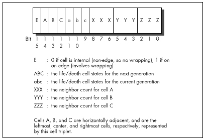
“The basic idea is to maintain a ‘change list.’ This is an array of pointers into the cell array. Each change list element points to a word which changes in the next generation. This way we don’t have to waste time scanning every cell since most of them do not change. Two passes are made through the change list. The first pass updates the cell display on the screen, sets the life/death status of each cell for this new generation, and updates the neighbor counts for the adjacent cells. There are some efficiencies gained by using cell triplets rather than individual cells since we usually don’t need to set all eight neighbors. [Again, the neighbor counts for cells in the same word are implied by the states of those cells.] The second pass sets the next-generation states for the cells and their neighbors, and in the process builds the change list for the next generation.
“Processing each word is a little complex but very fast. A 64K block of code exists with routines on each 256-byte boundary. Generally speaking, the entry point corresponds to the high byte of the cell word. This byte contains the life/death values and a bit to indicate if this is an edge condition. During the first pass we take the cell triplet word, AND it with 0XFE00, and jump to that address. During the second pass we take the cell triplet word, AND it with 0xFE00, OR it with 0x0100, and jump to that address. [Therefore, there are 128 possible jump targets on the first pass, and 128 more on the second, all on 256-byte boundaries and all keyed off the high 7 bits of the cell triplet state; because bit 8 of the jump index is 0 on the first pass and 1 on the second, there is no conflict. The lower bit isn’t needed for other purposes because only the edge flag bit and the six life/death state bits matter for jumping into David’s state machine. The other nine bits, the bits used for the neighbor counts, are used only in the next step.]
“Determining which changes must be made to a cell triplet is easy and
surprisingly quick. There’s no counting! Instead, I use a 64K lookup
table indexed by the cell triplet itself. The value of the lookup table
entry is equal to what the high byte should be in the next generation.
If this value is equal to the current high byte, then no changes are
necessary to the cell. Otherwise it is placed in the change list. Look
at the code in the Test() and Fix() functions
to see how this is done.” [This step is as important as it is obscure.
David has a 64K table organized so that if you use a word describing a
cell triplet as a lookup index, the byte you will read will be the state
of the high byte for the next generation. In other words, David’s table
is constructed so that the edge flag bit, the life/death states, and the
three neighbor count fields form an index to a byte describing the next
generation state for that triplet. In practice, only the next generation
field of the cell changes. Then, if another change to a nearby cell
tries to nudge that cell into changing again, David’s code sees that the
desired state is already set, and does not add that cell to the change
list again.]
Segment usage in David’s assembly code is summarized in Listing 18.6.
LISTING 18.6 QLIFE Assembly Segment Usage
CS : 64K code (table of routines on 256 byte boundaries)
DS : DGROUP (1st pass) / 64K cell life/death classification table (second pass)
ES : Change list
SS : DGROUP; the life cell grid and row/column table
FS : Video segment
GS : UnusedA Layperson’s Overview of QLIFE
Most likely, you’re scratching your head right now in bemusement. I don’t blame you; I felt the same way myself at first. It’s actually pretty simple, though, once you have the hang of it. Basically, David runs down the change list, visiting every cell that’s due to change in this generation, setting it to the new state, drawing it in the new state, and adjusting the counts of all its neighbors. David has a separate assembly routine for every possible change of state for a cell triplet, and he jumps to the proper routine by taking the cell triplet word, masking off the lower 9 bits, and jumping to the address where the appropriate code to perform that particular change of state resides. He does this for every entry in the change list. When this is completed, the current generation has been drawn and updated.
Now David runs down the change list again to generate the change list for the next generation. In this case, for every changed cell triplet, David looks at that triplet and all affected neighbors to see which will change in the next generation. He tests for this condition by using each potentially changed cell triplet word as an index into the aforementioned lookup table of new states. If the current state matches the appropriate state for the next generation, then there’s nothing to do and the cell is not added to the change list. If the states don’t match, then the cell is added to the change list, and the appropriate state for the next generation is set in the cell triplet. David checks the minimum possible number of cells for change by branching to code that checks only the relevant cells around each cell triplet in the current change list; that branching is accomplished by taking the cell triplet word, masking off the lower 9 bits, setting bit 8 to a 1-bit, and branching to the routine at that address. As with everything in this amazing program, this represents the least possible work to accomplish the desired result—just three instructions:
mov dh,[bp+1]
or dh,1
jmp dxThese suffice to select the proper, minimum-work code to process the next cell triplet that has changed, and all potentially affected neighbors. For all the size of David’s code, it has an astonishing economy of effort, as execution glides through the change list without a wasted instruction.
Alas, I don’t have the room to discuss Peter Klerings’ equally remarkable Life implementation here. I’ll close this chapter with a quote from Terje Mathisen, one of the finest optimizers it has ever been my pleasure to meet, who, after looking over David’s and Peter’s entries, said, “This has been an eye-opening experience for me. I honestly thought I had the fastest possible approach.” TANSTATFC.
There Ain’t No Such Thing As the Fastest Code.
Chapter 19 – Pentium: Not the Same Old Song
Learning a Whole Different Set of Optimization Rules
I can still remember the day I did my first 8088 programming. I had just moved over from the distantly related Z80, so the 8088 wasn’t totally alien, but it was nonetheless an incredibly exciting processor. The 8088’s instruction set was vastly more powerful and varied than the Z80’s, and as someone who thrives on puzzles of all sorts, from crosswords to Freecell to jigsaws to assembly language optimization, I was delighted to find that the 8088 made the optimization universe an order of magnitude more complicated—and correspondingly more interesting.
Well, the years went by and the Z80 just died, and 8088 optimization got ever more complex and intriguing as I discovered the hazards of the 8088’s cycle-eaters. By the time 1989 rolled around, I had written Zen of Assembly Language, in which I described all that I had learned about the 8088 and concluded that 8088 optimization was a black art of infinite subtlety. Unfortunately, by that time the 286 was the standard, with the 386 coming on strong, and if the 286 was less amenable to hand optimization than the 8088 (and it surely was), then the 386 was downright unfriendly. Sure, assembly optimization could buy some performance on the 386, but only 20, 30, 40 percent or so—a far cry from the 100 to 400 percent of the 8088. At the same time, compiler technology was improving quickly, and the days of hand tuning seemed numbered.
Happily, the 486 traveled to the beat of a different drum. The 486 had some interesting internal pipeline hazards, as well as an internal cache that made cycle counting more meaningful than ever before, and careful code massaging sometimes yielded startling results. Nonetheless, the 486 was still too simple to mark a return to the golden age of optimization.
The Return of Optimization as Art
Then the Pentium came around, and filled our code with optimization hazards, and life was good again. The Pentium has two execution pipelines and enough rules and exceptions to those rules to bring joy to the heart of the hardest-core assembly junkie. For a change, Intel documented most of the Pentium optimization rules and spread the word about them, so we don’t have to go through as much spelunking of the Pentium as with its predecessors. They’ve done this, I suspect, largely because more than any previous x86 processor, the Pentium’s performance is highly dependent on properly optimized code.
In the worst case, where the second execution pipe is dormant most of the time, the Pentium won’t perform all that much better than a 486 at the same clock speed. In the best case, where the second pipe is heavily used and the Pentium’s other advantages (such as branch prediction, write-back cache, 64-bit full speed external bus, and dual 8K caches) can kick in, the Pentium can be more than twice as fast as a 486. In a critical inner loop, hand optimization can double or even triple performance over 486-optimized code—and that’s on top of the sorts of algorithmic and design optimizations that are routinely performed on any processor. Good compilers can make a big difference on the Pentium, too, but there are some gotchas there, to which I’ll return later.
It’s been a long time coming, but hard-core, big-payoff assembly language optimization is back in style, and for the rest of this book I’ll be delving into the Byzantine wonders of the Pentium. In this chapter, I’ll do a quick overview, then cover a variety of smaller Pentium optimization topics. In the next chapter, I’ll tackle the 900-pound gorilla of Pentium optimization: superscalar (dual execution pipe) programming. Trust me, this’ll be fun.
Listen, do you want to know a secret? This lead-in has been brought to you with the help of “classic rock”—another way of saying “music Baby Boomers listened to back when they cared more about music than 401Ks and regular flossing.” There are so many of us Boomers that our music, even the worst of it, will never go away. When we’re 90 years old, propped up in our Kraftmatic adjustable beds and surfing the 5,000-channel information superhighway from one infomercial to the next, the sound system in the retirement community will be piping in a Muzak version of “Louie, Louie,” while on the holovid Country Joe McDonald and the Fish pitch Preparation H. I can hardly wait.
Gimme a “P”….
The Pentium: An Overview
Architecturally, the Pentium is vastly different in many ways from the 486, but most of those differences are transparent to programmers. After all, the whole idea behind the Pentium is that it runs the same code as previous x86 processors, but faster; otherwise, Intel could have made a faster, cheaper RISC processor. Still, knowledge of the Pentium’s architecture is useful for understanding exactly how code will perform, and a few of the architectural differences are most decidedly not transparent to performance programmers.
The Pentium is essentially one full 486 execution unit (EU), plus a
second stripped-down 486 EU, on a single chip. The first EU is referred
to as the U execution pipe, or U-pipe; the second, more limited
one is called the V-pipe. The two pipes are capable of
executing instructions simultaneously, have separate write buffers, and
can even access the data cache simultaneously (although with certain
limitations that I’ll discuss in the next chapter), so on the Pentium it
is possible to execute two instructions, even instructions that access
memory, in a single clock. The cycle times for instruction execution in
a given pipe (both pipes process instructions at the same speed) are
comparable to those for the 486, although some instructions—notably
MUL, the repeated string instructions, and some of the
shifts and rotates—have gotten faster.
My first thought upon hearing of the Pentium’s dual pipes was to wonder how often the prefetch queue stalls for lack of instruction bytes, given that the demand for instruction bytes can be twice that of the 486. The answer is: rarely indeed, and then only because the code is not in the internal cache. The 486 has a single 8K cache that stores both code and data, and prefetching can stall if data fetching doesn’t allow time for prefetching to occur (although this rarely happens in practice).
(And yes, self-modifying code still works; as with all Pentium changes, the dual caches introduce no incompatibilities with 386/486 code.) Also, because the code and data caches are separate, code can’t be driven out of the cache in a tight loop that accesses a lot of data, unlike the 486. In addition, the Pentium expands the 486’s 32-byte prefetch queue to 128 bytes. In conjunction with the branch prediction feature (described next), which allows the Pentium to prefetch properly at most branches, this larger prefetch queue means that the Pentium’s two pipes should be better fed than those of any previous x86 processor.
Crossing Cache Lines
There are three other characteristics of the Pentium that make for a healthy supply of instruction bytes. One is that the Pentium can prefetch instructions across cache lines. Unlike the 486, where there is a 3-cycle penalty for branching to an instruction that spans a cache line, there’s no such penalty on the Pentium. The second is that the cache line size (the number of bytes fetched from the external cache or main memory on a cache miss) on the Pentium is 32 bytes, twice the size of the 486’s cache line, so a cache miss causes a longer run of instructions to be placed in the cache than on the 486. The third is that the Pentium’s external bus is twice as wide as the 486’s, at 64 bits, and runs twice as fast, at 66 MHz, so the Pentium can fetch both instruction and data bytes from the external cache four times as fast as the 486.
The upshot of all this is that at the same clock speed, with code and data that are mostly in the internal caches, the Pentium maxes out somewhere around twice as fast as a 486. (When the caches are missed a lot, the Pentium can get as much as three to four times faster, due to the superior external bus and bigger caches.) Most of this won’t affect how you program, but it is useful to know that you don’t have to worry about instruction fetching. It’s also useful to know the sizes of the caches because a high cache hit rate is crucial to Pentium performance. Cache misses are vastly slower than cache hits (anywhere from two to 50 or more times as slow, depending on the speed of the external cache and whether the external cache misses as well), and the Pentium can’t use the V-pipe on code that hasn’t already been executed out of the cache at least once. This means that it is very important to get the working sets of critical loops to fit in the internal caches.
One change in the Pentium that you definitely do have to worry about is superscalar execution. Utilization of the V-pipe can range from near zero percent to 100 percent, depending on the code being executed, and careful rearrangement of code can have amazing effects. Maxing out V-pipe use is not a trivial task; I’ll spend all of the next chapter discussing it so as to have time to cover it properly. In the meantime, two good references for superscalar programming and other Pentium information are Intel’s Pentium Processor User’s Manual: Volume 3: Architecture and Programming Manual (ISBN 1-55512-195-0; Intel order number 241430-001), and the article “Optimizing Pentium Code” by Mike Schmidt, in Dr. Dobb’s Journal for January 1994.
Cache Organization
There are two other interesting changes in the Pentium’s cache organization. First, the cache is two-way set-associative, whereas the 486 is four-way set-associative. The details of this don’t matter, but simply put, this, combined with the 32-byte cache line size, means that the Pentium has somewhat coarser granularity in both space and time than the 486 in terms of packing bytes into the cache, although the total cache space is now bigger. There’s nothing you can do about this, but it may make it a little harder to get a loop’s working set into the cache. Second, the internal cache can now be configured (by the BIOS or OS; you won’t have to worry about it) for write-back rather than write-through operation. This means that writes to the internal data cache don’t necessarily get propagated to the external bus until other demands for cache space force the data out of the cache, making repeated writes to memory variables such as loop counters cheaper on average than on the 486, although not as cheap as registers.
As a final note on Pentium architecture for this chapter, the pipeline stalls (what Intel calls AGIs, for Address Generation Interlocks) that I discussed earlier in this book (see Chapter 12) are still present in the Pentium. In fact, they’re there in spades on the Pentium; the two pipelines mean that an AGI can now slow down execution of an instruction that’s three instructions away from the AGI (because four instructions can execute in two cycles). So, for example, the code sequence
add edx,4 ;U-pipe cycle 1
mov ecx,[ebx] ;V-pipe cycle 1
add ebx,4 ;U-pipe cycle 2
mov [edx],ecx ;V-pipe cycle 3
; due to AGI
; (would have been
; V-pipe cycle 2)takes three cycles rather than the two cycles it should take, because EDX was modified on cycle 1 and an attempt was made to use it on cycle two, before the AGI had time to clear—even though there are two instructions between the instructions that are actually involved in the AGI. Rearranging the code like
mov ecx,[ebx] ;U-pipe cycle 1
add ebx,4 ;V-pipe cycle 1
mov [edx+4],ecx ;U-pipe cycle 2
add edx,4 ;V-pipe cycle 2makes it functionally identical, but cuts the cycles to 2—a 50 percent improvement. Clearly, avoiding AGIs becomes a much more challenging and rewarding game in a superscalar world, one to which I’ll return in the next chapter.
Faster Addressing and More
I’ll spend the rest of this chapter covering a variety of Pentium
optimization tips. For starters, effective address calculations (that
is, the addition and scaling required to calculate a memory operand’s
address, as for example in MOV EAX,[EBX+ECX*2+4]) never
take any extra cycles on the Pentium (other than possibly an AGI cycle),
even for the use of base+index addressing (as in
MOV [ESI+EDI],EAX) or scaling (*2, *4, or *8, as in
INC ARRAY[ESI*4]). On the 486, both of the latter cases
cause a 1-cycle penalty. The faster effective address calculations have
the side effect of making LEA very attractive as an
arithmetic instruction. LEA can add any two registers, one
of which can be multiplied by one, two, four, or eight, plus a constant
value, and can store the result in any register—all in one cycle, apart
from AGIs. Not only that, but as we’ll see in the next chapter,
LEA can go through either pipe, whereas SHL
can only go through the U-pipe, so LEA is often a superior
choice for multiplication by three, four, five, eight, or nine.
(ADD is the best choice for multiplication by two.) If you
use LEA for arithmetic, do remember that unlike
ADD and SHL, it doesn’t modify any flags.
As on the 486, memory operands should not cross any more alignment boundaries than absolutely necessary. Word operands should be word-aligned, dword operands should be dword-aligned, and qword operands (double-precision variables) should be qword-aligned. Spanning a dword boundary, as in
mov ebx,3
:
mov eax,[ebx]costs three cycles. On the other hand, as noted above, branch targets can now span cache lines with impunity, so on the Pentium there’s no good argument for the paragraph (that is, 16-byte) alignment that Intel recommends for 486 jump targets. The 32-byte alignment might make for slightly more efficient Pentium cache usage, but would make code much bigger overall.
Instruction prefixes are awfully expensive; avoid them if you can.
(These include size and addressing prefixes, segment overrides,
LOCK, and the 0FH prefixes that extend the instruction set
with instructions such as MOVSX. The exceptions are
conditional jumps, a fast special case.) At a minimum, a prefix byte
generally takes an extra cycle and shuts down the V-pipe for that cycle,
effectively costing as much as two normal instructions (although prefix
cycles can overlap with previous multicycle instructions, or AGIs, as on
the 486). This means that using 32-bit addressing or 32-bit operands in
a 16-bit segment, or vice versa, makes for bigger code that’s
significantly slower. So, for example, you should generally avoid 16-bit
variables (shorts, in C) in 32-bit code, although if using 32-bit
variables where they’re not needed makes your data space get a lot
bigger, you may want to stick with shorts, especially since longs use
the cache less efficiently than shorts. The trade-off depends on the
amount of data and the number of instructions that reference that data.
(eight-bit variables, such as chars, have no extra overhead and can be
used freely, although they may be less desirable than longs for
compilers that tend to promote variables to longs when performing
calculations.) Likewise, you should if possible avoid putting data in
the code segment and referring to it with a CS: prefix, or otherwise
using segment overrides.
LOCK is a particularly costly instruction, especially on
multiprocessor machines, because it locks the bus and requires that the
hardware be brought into a synchronized state. The cost varies depending
on the processor and system, but LOCK can make an
INC [*mem*] instruction (which normally takes 3 cycles) 5,
10, or more cycles slower. Most programmers will never use
LOCK on purpose—it’s primarily an operating system
instruction—but there’s a hidden gotcha here because the
XCHG instruction always locks the bus when used with a
memory operand.
XCHGis a tempting instruction that’s often used in assembly language; for example, exchanging with video memory is a popular way to read and write VGA memory in a single instruction—but it’s now a bad idea. As it happens, on the 486 and Pentium, usingMOVs to read and write memory is faster, anyway; and even on the 486, my measurements indicate a five-cycle tax forLOCKin general, and a nine-cycle execution time forXCHGwith memory. AvoidXCHGwith memory if you possibly can.
As with the 486, don’t use ENTER or LEAVE,
which are slower than the equivalent discrete instructions. Also, start
using TEST *reg,reg* instead of AND *reg,reg*
or OR *reg,reg* to test whether a register is zero. The
reason, as we’ll see in Chapter 21, is that TEST, unlike
AND and OR, never modifies the target
register. Although in this particular case AND and
OR don’t modify the target register either, the Pentium has
no way of knowing that ahead of time, so if AND or
OR goes through the U-pipe, the Pentium may have to shut
down the V-pipe for a cycle to avoid potential dependencies on the
result of the AND or OR. TEST
suffers from no such potential dependencies.
Branch Prediction
One brand-spanking-new feature of the Pentium is branch prediction, whereby the Pentium tries to guess, based on past history, which way (or, for conditional jumps, whether or not), your code will jump at each branch, and prefetches along the likelier path. If the guess is correct, the branch or fall-through takes only 1 cycle—2 cycles less than a branch and the same as a fall-through on the 486; if the guess is wrong, the branch or fall-through takes 4 or 5 cycles (if it executes in the U- or V-pipe, respectively)—1 or 2 cycles more than a branch and 3 or 4 cycles more than a fall-through on the 486.
Also, unrolled loops are bigger than normal loops, so there are extra (and expensive) cache misses the first time through the loop if the entire loop isn’t already in the cache; then, too, an unrolled loop will shoulder other code out of the internal and external caches. If in a critical loop you absolutely need the time taken by the loop control instructions, or if you need an extra register that can be freed by unrolling a loop, then by all means unroll the loop. Don’t expect the sort of speed-up you get from this on the 486 or especially the 386, though, and watch out for the cache effects.
You may well wonder exactly when the Pentium correctly predicts branching. Alas, this is one area that Intel has declined to document, beyond saying that you should endeavor to fall through branches when you have a choice. That’s good advice on every other x86 processor, anyway, so it’s well worth following. Also, it’s a pretty safe bet that in a tight loop, the Pentium will start guessing the right branch direction at the bottom of the loop pretty quickly, so you can treat loop branches as one-cycle instructions.
It’s an equally safe bet that it’s a bad move to have in a loop a conditional branch that goes both ways on a random basis; it’s hard to see how the Pentium could consistently predict such branches correctly, and mispredicted branches are more expensive than they might appear to be. Not only does a mispredicted branch take 4 or 5 cycles, but the Pentium can potentially execute as many as 8 or 10 instructions in that time—3 times as many as the 486 can execute during its branch time—so correct branch prediction (or eliminating branch instructions, if possible) is very important in inner loops. Note that on the 486 you can count on a branch to take 1 cycle when it falls through, but on the Pentium you can’t be sure whether it will take 1 or either 4 or 5 cycles on any given iteration.
Miscellaneous Pentium Topics
The Pentium has all the instructions of the 486, plus a few new ones.
One much-needed instruction that has finally made it into the
instruction set is CPUID, which allows your code to
determine what processor it’s running on. CPUID is 15 years
late, but at least it’s finally here. Another new instruction is
CMPXCHG8B, which does a compare and conditional exchange on
a qword. CMPXCHG8B doesn’t seem to me to be a particularly
useful instruction, but I’m sure Intel wouldn’t have added it without a
reason; if you know of a use for it, please pass it along to me.
486 versus Pentium Optimization
Many Pentium optimizations help, or at least don’t hurt, on the 486. Many, but not all—and many do hurt on the 386. As I discuss various Pentium optimizations, I will attempt to note the effects on the 486 as well, but doing this in complete detail would double the sizes of these discussions and make them hard to follow. In general, I’d recommend reserving Pentium optimization for your most critical code, and even there, it’s a good idea to have at least two code paths, one for the 386 and one for the 486/Pentium. It’s also a good idea to time your code on a 486 before and after Pentium-optimizing it, to make sure you haven’t hurt performance on what will be, after all, by far the most important processor over the next couple of years.
With that in mind, is optimizing for the Pentium even worthwhile today? That depends on your application and its market—but if you want absolutely the best possible performance for your DOS and Windows apps on the fastest hardware, Pentium optimization can make your code scream.
Going Superscalar
In the next chapter, we’ll look into the single biggest element of Pentium performance, cranking up the Pentium’s second execution pipe. This is the area in which compiler technology is most touted for the Pentium, the two thoughts apparently being that (1) most existing code is in C, so recompiling to use the second pipe better is an automatic win, and (2) it’s so complicated to optimize Pentium code that only a compiler can do it well. The first point is a reasonable one, but it does suffer from one flaw for large programs, in that Pentium-optimized code is larger than 486- or 386-optimized code, for reasons that will become apparent in the next chapter. Larger code means more cache misses and more page faults; and while most of the code in any program is not critical to performance, compilers optimize code indiscriminately.
The result is that Pentium compiler optimization not only expands code, but can be less beneficial than expected or even slower in some cases. What makes more sense is enabling Pentium optimization only for key code. Better yet, you could hand-tune the most important code—and yes, you can absolutely do a better job with a small, critical loop than any PC compiler I’ve ever seen, or expect to see. Sure, you keep hearing how great each new compiler generation is, and compilers certainly have improved; but they play by the same rules we do, and we’re more flexible and know more about what we’re doing—and now we have the wonderfully complex and powerful Pentium upon which to loose our carbon-based optimizers.
A compiler that generates better code than a good assembly programmer? That’ll be the day.
Chapter 20 – Pentium Rules
How Your Carbon-Based Optimizer Can Put the “Super” in Superscalar
At the 1983 West Coast Computer Faire, my friend Dan Illowsky, Andy Greenberg (co-author of Wizardry, at that time the best-selling computer game ever), and I had an animated discussion about starting a company in the then-budding world of microcomputer software. One hot new software category at the time was educational software, and one of the hottest new educational software companies was Spinnaker Software. Andy used Spinnaker as an example of a company that had been aimed at a good market and started up properly, and was succeeding as a result. Dan didn’t buy this; his point was that Spinnaker had been given a bundle of money to get off the ground, and was growing only by spending a lot of that money in order to move its products. “Heck,” said Dan, “I could get that kind of market share too if I gave away a fifty-dollar bill with each of my games.”
Remember, this was a time when a program, two diskette drives (for duplicating disks), and a couple of ads were enough to start a company, and, in fact, Dan built a very successful game company out of not much more than that. (I’ll never forget coming to visit one day and finding his apartment stuffed literally to the walls and ceiling with boxes of diskettes and game packages; he had left a narrow path to the computer so his wife and his mother could get in there to duplicate disks.) Back then, the field was wide open, with just about every competent programmer thinking of striking out on his or her own to try to make their fortune, and Dan and Andy and I were no exceptions. In short, we were having a perfectly normal conversation, and Dan’s comment was both appropriate, and, in retrospect, accurate.
Appropriate, save for one thing: We were having this conversation while walking through a low-rent section of Market Street in San Francisco at night. A bum sitting against a nearby building overheard Dan, and rose up, shouting in a quavering voice loud enough to wake the dead, “Fifty-dollar bill! Fifty-dollar bill! He’s giving away fifty-dollar bills!” We ignored him; undaunted, he followed us for a good half mile, stopping every few feet to bellow “fifty-dollar bill!” No one else seemed to notice, and no one hassled us, but I was mighty happy to get to the sanctuary of the Fairmont Hotel and slip inside.
The point is, most actions aren’t inherently good or bad; it’s all a matter of context. If Dan had uttered the words “fifty-dollar bill” on the West Coast Faire’s show floor, no one would have batted an eye. If he had said it in a slightly worse part of town than he did, we might have learned just how fast the three of us could run.
Similarly, there’s no such thing as inherently fast code, only fast
code in context. At the moment, the context is the Pentium, and the
truth is that a sizable number of the x86 optimization tricks that you
and I have learned over the past ten years are obsolete on the Pentium.
True, the Pentium contains what amounts to about one-and-a-half 486s,
but, as we’ll see shortly, that doesn’t mean that optimized Pentium code
looks much like optimized 486 code, or that fast 486 code runs
particularly well on a Pentium. (Fast Pentium code, on the other hand,
does tend to run well on the 486; the only major downsides are that it’s
larger, and that the FXCH instruction, which is largely
free on the Pentium, is expensive on the 486.) So discard your x86
preconceptions as we delve into superscalar optimization for this
one-of-a-kind processor.
An Instruction in Every Pipe
In the last chapter, we took a quick tour of the Pentium’s architecture, and started to look into the Pentium’s optimization rules. Now we’re ready to get to the key rules, those having to do with the Pentium’s most unique and powerful feature, the ability to execute more than one instruction per cycle. This is known as superscalar execution, and has heretofore been the sole province of fast RISC CPUs. The Pentium has two integer execution units, called the U-pipe and the V-pipe, which can execute two separate instructions simultaneously, potentially doubling performance—but only under the proper conditions. (There is also a separate floating-point execution unit that I won’t have the space to cover in this book.) Your job, as a performance programmer, is to understand the conditions needed for superscalar performance and make sure they’re met, and that’s what this and the next chapters are all about.
The two pipes are not independent processors housed in a single chip; that is, the Pentium is not like having two 486s in a single computer. Rather, the two pipes are integral, parallel parts of the same processor. They operate on the same instruction stream, with the V-pipe simply executing the next instruction that the U-pipe would have handled, as shown in Figure 20.1. What the Pentium does, pure and simple, is execute a single instruction stream and, whenever possible, take the next two waiting instructions and execute both at once, rather than one after the other.
The U-pipe is the more capable of the two pipes, able to execute any
instruction in the Pentium’s instruction set. (A number of instructions
actually use both pipes at once. Logically, though, you can think of
such instructions as U-pipe instructions, and of the Pentium
optimization model as one in which the U-pipe is able to execute all
instructions and is always active, with the objective being to keep the
V-pipe also working as much of the time as possible.) The U-pipe is
generally similar to a full 486 in terms of both capabilities and
instruction cycle counts. The V-pipe is a 486 subset, able to execute
simple instructions such as MOV and ADD, but
unable to handle MUL, DIV, string instructions, any sort of
rotation or shift, or even ADC or SBB.
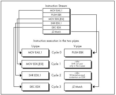
Getting two instructions executing simultaneously in the two pipes is
trickier than it sounds, not only because the V-pipe can handle only a
relatively small subset of the Pentium’s instruction set, but also
because those instructions that the V-pipe can handle are able to pair
only with certain U-pipe instructions. For example, MOVSD
uses both pipes, so no instruction can be executed in parallel with
MOVSD.
MOVSDnearly twice as fast on the Pentium as on the 486, but it’s nonetheless slower than using equivalent simpler instructions that allow for superscalar execution. Stick to the Pentium’s RISC-like instructions—the pairable instructions I’ll discuss next—when you’re seeking maximum performance, with just a few exceptions such asREP MOVSandREP STOS.
Trickier yet, register contention can shut down the V-pipe on any given cycle, and Address Generation Interlocks (AGIs) can stall either pipe at any time, as we’ll see in the next chapter.
The key to Pentium optimization is to view execution as a stream of instructions going through the U- and V-pipes, and to eliminate, as much as possible, instruction mixes that take the V-pipe out of action. In practice, this is not too difficult. The only hard part is keeping in mind the long list of rules governing instruction pairing. The place to begin is with the set of instructions that can go through the V-pipe.
V-Pipe-Capable Instructions
Any instruction can go through the U-pipe, and, for practical
purposes, the U-pipe is always executing instructions. (The exceptions
are when the U-pipe execution unit is waiting for instruction or data
bytes after a cache miss, and when a U-pipe instruction finishes before
a paired V-pipe instruction, as I’ll discuss below.) Only the
instructions shown in Table 20.1 can go through the V-pipe. In addition,
the V-pipe can execute a separate instruction only when one of the
instructions listed in Table 20.2 is executing in the U-pipe;
superscalar execution is not possible while any instruction not listed
in Table 20.2 is executing in the U-pipe. So, for example, if you use
SHR EDX,CL, which takes 4 cycles to execute, no other
instructions can execute during those 4 cycles; if, on the other hand,
you use SHR EDX,10, it will take 1 cycle to execute in the
U-pipe, and another instruction can potentially execute concurrently in
the V-pipe. (As you can see, similar instruction sequences can have
vastly different performance characteristics on the Pentium.)
Basically, after the current instruction or pair of instructions is finished (that is, once neither the U- nor V-pipe is executing anything), the Pentium sends the next instruction through the U-pipe. If the instruction after the one in the U-pipe is an instruction the V-pipe can handle, if the instruction in the U-pipe is pairable, and if register contention doesn’t occur, then the V-pipe starts executing that instruction, as shown in Figure 20.2. Otherwise, the second instruction waits until the first instruction is done, then executes in the U-pipe, possibly pairing with the next instruction in line if all pairing conditions are met.
MOV reg,reg (1 cycle)
mem,reg (1 cycle)
reg,mem (1 cycle)
reg,immediate (1 cycle)
mem,immediate (1 cycle)†
AND/OR/XOR/ADD/SUB reg,reg (1 cycle)
mem,reg (3 cycles)
reg,mem (2 cycles)
reg,immediate (1 cycle)
mem,immediate (3 cycles)†
INC/DEC reg (1 cycle)
mem (3 cycles)
CMP reg,reg (1 cycle)
mem,reg (2 cycles)
reg,mem (2 cycles)
reg,immediate (1 cycle)
mem,immediate (2 cycles)†
TEST reg,reg (1 cycle)
EAX,immediate (1 cycle)
PUSH/POP reg (1 cycle)
immediate (1 cycle)
LEA reg,mem (1 cycle)
JCC near (1 cycle if predicted correctly;
5 cycles otherwise in V-pipe,
4 cycles otherwise in U-pipe)
JMP/CALL near (1 cycle if predicted correctly;
3 cycles otherwise)† Can’t execute in V-pipe if address contains a displacement
Table 20.1 Instructions that can execute in the V-pipe.
The list of instructions the V-pipe can handle is not very long, and the list of U-pipe pairable instructions is not much longer, but these actually constitute the bulk of the instructions used in PC software. As a result, a fair amount of pairing happens even in normal, non-Pentium-optimized code. This fact, plus the 64-bit 66 MHz bus, branch prediction, dual 8K internal caches, and other Pentium features, together mean that a Pentium is considerably faster than a 486 at the same clock speed, even without Pentium-specific optimization, contrary to some reports.
Besides, almost all operations can be performed by combinations of
pairable instructions. For example, PUSH [*mem*] is not on
either list, but both MOV *reg*,[*mem*] and
PUSH *reg* are, and those two instructions can be used to
push a value stored in memory. In fact, given the proper instruction
stream, the discrete instructions can perform this operation effectively
in just 1 cycle (taking one-half of each of 2 cycles, for 2*0.5 = 1
cycle total execution time), as shown in Figure 20.3—a full cycle
faster than PUSH [*mem*], which takes 2
cycles.
MOV reg,reg (1 cycle)
mem,reg (1 cycle)
reg,mem (1 cycle)
reg,immediate (1 cycle)
mem,immediate (1 cycle)†
AND/OR/XOR/ADD/SUB/ADC/SBB reg,reg (1 cycle)
mem,reg (3 cycles)
reg,mem (2 cycles)
reg,immediate (1 cycle)
mem,immediate (3 cycles)†
INC/DEC reg (1 cycle)
mem (3 cycles)
CMP reg,reg (1 cycle)
mem,reg (2 cycles)
reg,mem (2 cycles)
reg,immediate (1 cycle)
mem,immediate (2 cycles)†
TEST reg,reg (1 cycle)
EAX,immediate (1 cycle)
PUSH/POP reg (1 cycle)
immediate (1 cycle)
LEA reg,mem (1 cycle)
SHL/SHR/SAL/SAR reg,immediate (1 cycle)††
ROL/ROR/RCL/RCR reg,1 (1 cycle)† Can’t pair if address contains a displacement
†† Includes shift-by-1 forms of instructions
Table 20.2 Instructions that, when executed in the U-pipe, allow V-pipe-executable instructions to execute simultaneously (pair) in the V-pipe.
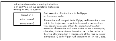
One downside of this “RISCification” (turning complex instructions into simple, RISC-like ones) of Pentium-optimized code is that it makes for substantially larger code. For example,
push dword ptr [esi]is one byte smaller than this sequence:
mov eax,[esi]
push eax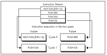
A more telling example is the following
add [MemVar],eaxversus the equivalent:
mov edx,[MemVar]
add edx,eax
mov [MemVar],edxThe single complex instruction takes 3 cycles and is 6 bytes long;
with proper sequencing, interleaving the simple instructions with other
instructions that don’t use EDX or Mem Var, the
three-instruction sequence can be reduced to 1.5 cycles, but it is
14 bytes long.
Lockstep Execution
You may wonder why anyone would bother breaking
ADD [MemVar],EAX into three instructions, given that this
instruction can go through either pipe with equal ease. The answer is
that while the memory-accessing instructions other than
MOV, PUSH, and POP listed in Table 20.1 (that
is,
INC/DEC [*mem*], ADD/SUB/XOR/AND/OR/CMP/ADC/SBB *reg*,[*mem*],
and ADD/SUB/XOR/AND/OR/CMP/ADC/SBB [*mem*],*reg/immed*) can
be paired, they do not provide the 100 percent overlap that we seek. If
you look at Tables 20.1 and 20.2, you will see that instructions taking
from 1 to 3 cycles can pair. However, any pair of instructions goes
through the two pipes in lockstep. This means, for example, that if
ADD [EBX],EDX is going through the U-pipe, and
INC EAX is going through the V-pipe, the V-pipe will be
idle for 2 of the 3 cycles that the U-pipe takes to execute its
instruction, as shown in Figure 20.4. Out of the theoretical 6 cycles of
work that can be done during this time, we actually get only 4 cycles of
work, or 67 percent utilization. Even though these instructions pair,
then, this sequence fails to make maximum use of the Pentium’s
horsepower.
The key here is that when two instructions pair, both execution units are tied up until both instructions have finished (which means at least for the amount of time required for the longer of the two to execute, plus possibly some extra cycles for pairable instructions that can’t fully overlap, as described below). The logical conclusion would seem to be that we should strive to pair instructions of the same lengths, but that is often not correct.
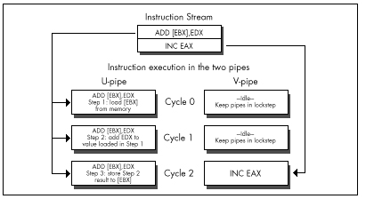
Here’s why. The Pentium is fully capable of handling instructions that use memory operands in either pipe, or, if necessary, in both pipes at once. Each pipe has its own write FIFO, which buffers the last few writes and takes care of writing the data out while the Pentium continues processing. The Pentium also has a write-back internal data cache, so data that is frequently changed doesn’t have to be written to external memory (which is much slower than the cache) very often. This combination means that unless you write large blocks of data at a high speed, the Pentium should be able to keep up with both pipes’ memory writes without stalling execution.
The Pentium is also designed to satisfy both pipes’ needs for reading memory operands with little waiting. The data cache is constructed so that both pipes can read from the cache on the same cycle. This feat is accomplished by organizing the data cache as eight-banked memory, as shown in Figure 20.5, with each 32-byte cache line consisting of 8 dwords, 1 in each bank. The banks are independent of one another, so as long as the desired data is in the cache and the U- and V-pipes don’t try to read from the same bank on the same cycle, both pipes can read memory operands on the same cycle. (If there is a cache bank collision, the V-pipe instruction stalls for one cycle.)
Normally, you won’t pay close attention to which of the eight dword banks your paired memory accesses fall in—that’s just too much work—but you might want to watch out for simultaneously read addresses that have the same values for address
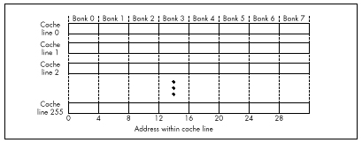
bits 2, 3, and 4 (fall in the same bank) in tight loops, and you should also avoid sequences like
mov bl,[esi]
mov bh,[esi+1]because both operands will generally be in the same bank. An alternative is to place another instruction between the two instructions that access the same bank, as in this sequence:
mov bl,[esi]
mov edi,edx
mov bh,[esi+1]By the way, the reason a code sequence that takes two instructions to load a single word is attractive in a 32-bit segment is because it takes only one cycle when the two instructions can be paired with other instructions; by contrast, the obvious way of loading BX
mov bx,[esi]takes 1.5 to two cycles because the size prefix can’t pair, as described below. This is yet another example of how different Pentium optimization can be from everything we’ve learned about its predecessors.
The problem with pairing non-single-cycle instructions arises when a
pipe executes an instruction other than MOV that has an
explicit memory operand. (I’ll call these complex memory
instructions. They’re the only pairable instructions, other than
branches, that take more than one cycle.) We’ve already seen that,
because instructions go through the pipes in lockstep, if one pipe
executes a complex memory instruction such as ADD EAX,[EBX]
while the other pipe executes a single-cycle instruction, the pipe with
the faster instruction will sit idle for part of the time, wasting
cycles. You might think that if both pipes execute complex instructions
of the same length, then neither would lie idle, but that turns out to
not always be the case. Two two-cycle instructions (instructions with
register destination operands) can indeed pair and execute in two
cycles, so it’s okay to pair two instructions such as these:
add esi,[SourceSkip] ;U-pipe cycles 1 and 2
add edi,[DestinationSkip] ;V-pipe cycles 1 and 2However, this beneficial pairing does not extend to
non-MOV instructions with explicit memory destination
operands, such as ADD [EBX],EAX. The Pentium executes
only one such memory instruction at a time; if two memory-destination
complex instructions get paired, first the U-pipe instruction is
executed, and then the V-pipe instruction, with only one cycle of
overlap, as shown in Figure 20.6. I don’t know for sure, but I’d guess
that this is to guarantee that the two pipes will never perform
out-of-order access to any given memory location. Thus, even though
AND [EBX],AL pairs with AND [ECX],DL, the two
instructions take 5 cycles in all to execute, and 4 cycles of idle
time—2 in the U-pipe and 2 in the V-pipe, out of 10 cycles in all—are
incurred in the process.
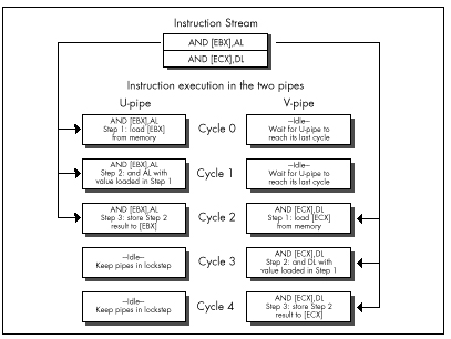
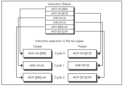
The solution is to break the instructions into simple instructions and interleave them, as shown in Figure 20.7, which accomplishes the same task in 3 cycles, with no idle cycles whatsoever. Figure 20.7 is a good example of what optimized Pentium code generally looks like: mostly one-cycle instructions, mixed together so that at least two operations are in progress at once. It’s not the easiest code to read or write, but it’s the only way to get both pipes running at capacity.
Superscalar Notes
You may well ask why it’s necessary to interleave operations, as is done in Figure 20.7. It seems simpler just to turn
and [ebx],alinto
mov dl,[ebx]
and dl,al
mov [ebx],dland be done with it. The problem here is one of dependency. Before
the Pentium can execute AND DL,AL,, it must first know what
is in DL, and it can’t know that until it loads DL from the address
pointed to by EBX. Therefore, AND DL,AL can’t happen until
the cycle after MOV DL,[EBX] executes. Likewise, the result
can’t be stored until the cycle after AND DL,AL has
finished. This means that these instructions, as written, can’t possibly
pair, so the sequence takes the same three cycles as
AND [EBX],AL. (Now it should be clear why
AND [EBX], AL takes 3 cycles.) Consequently, it’s necessary
to interleave these instructions with instructions that use other
registers, so this set of operations can execute in one pipe while the
other, unrelated set executes in the other pipe, as is done in Figure
20.7.
What we’ve just seen is the read-after-write form of the superscalar hazard known as register contention. I’ll return to the subject of register contention in the next chapter; in the remainder of this chapter I’d like to cover a few short items about superscalar execution.
Register Starvation
The above examples should make it pretty clear that effective superscalar programming puts a lot of strain on the Pentium’s relatively small register set. There are only seven general-purpose registers (I strongly suggest using EBP in critical loops), and it does not help to have to sacrifice one of those registers for temporary storage on each complex memory operation; in pre-superscalar days, we used to employ those handy CISC memory instructions to do all that stuff without using any extra registers.
Also be aware that prefixes of every sort, with the sole exception of the 0FH prefix on non-short conditional jumps, always execute in the U-pipe, and that Intel’s documentation indicates that no pairing can happen while a prefix byte executes. (As I’ll discuss in the next chapter, my experiments indicate that this rule doesn’t always apply to multiple-cycle instructions, but you still won’t go far wrong by assuming that the above rule is correct and trying to eliminate prefix bytes.) A prefix byte takes one cycle to execute; after that cycle, the actual prefixed instruction itself will go through the U-pipe, and if it and the following instruction are mutually pairable, then they will pair. Nonetheless, prefix bytes are very expensive, effectively taking at least as long as two normal instructions, and possibly, if a prefixed instruction could otherwise have paired in the V-pipe with the previous instruction, taking as long as three normal instructions, as shown in Figure 20.8.
Finally, bear in mind that if the instructions being executed have
not already been executed at least once since they were loaded into the
internal cache, they can pair only if the first (U-pipe) instruction is
not only pairable but also exactly 1 byte long, a category that includes
only INC *reg*, DEC *reg*, PUSH *reg*, and
POP *reg*. Knowing this can help you understand why
sometimes, timing reveals that your code runs slower than it seems it
should, although this will generally occur only when the cache working
set for the code you’re timing is on the order of 8K or more—an awful
lot of code to try to optimize.
It should be excruciatingly clear by this point that you must time your Pentium-optimized code if you’re to have any hope of knowing if your optimizations are working as well as you think they are; there are just too many details involved for you to be sure your optimizations are working properly without checking. My most basic optimization rule has always been to grab the Zen timer and measure actual performance—and nowhere is this more true than on the Pentium. Don’t believe it until you measure it!
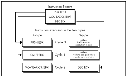
Chapter 21 – Unleashing the Pentium’s V-Pipe
Focusing on Keeping Both Pentium Pipes Full
The other day, my daughter suggested that we each draw the prettiest picture we could, then see whose was prettier. I won’t comment on who won, except to note that apparently a bolt of lightning zipping toward a moose with antlers that bear an unfortunate resemblance to a propeller beanie isn’t going to win me any scholarships to art school, if you catch my drift. Anyway, my drawing happened to feature the word “chartreuse” (because it rhymed with “moose” and “Zeus”—hence the lightning; more than that I am not at liberty to divulge), and she wanted to know if the moose was actually chartreuse. I had to admit that I didn’t know, so we went to the dictionary, whereupon we learned that chartreuse is a pale apple-green color. Then she brought up the Windows Control Panel, pointed to the selection of predefined colors, and asked, “Which of those is chartreuse?”—and I realized that I still didn’t know.
Some things can be described perfectly with words, but others just have to be experienced. Color is one such category, and Pentium optimization is another. I’ve spent the last two chapters detailing the rules for Pentium optimization, and I’ll spend half of this one doing so, as well. That’s good; without understanding the fundamentals, we have no chance of optimizing well. It’s not enough, though. We also need to look at a real-world example of Pentium optimization in action, and we’ll do that later in this chapter; after which, you should go out and do some Pentium optimization on your own. Optimization is one of those things that you can learn a lot about from reading, but ultimately it has to sink into your pores as you do it—especially Pentium optimization because the Pentium is perhaps the most complex (and rewarding) chip to optimize for that I’ve ever seen.
In the last chapter, we explored the dual-execution-pipe nature of the Pentium, and learned which instructions could pair (execute simultaneously) in which pipes. Now we’re ready to look at AGIs and register contention—two hazards that can prevent otherwise properly written code from taking full advantage of the Pentium’s two pipes, and can thereby keep your code from pushing the Pentium to maximum performance.
Address Generation Interlocks
The Pentium is advertised as having a five-stage pipeline for each of its execution units. All this means is that at any given time, up to five instructions are in various stages of execution in each pipe; this overlapping of execution is done for speed, so each instruction doesn’t have to wait until the previous one has finished. The only way that the Pentium’s pipelining directly affects the way you program is in the areas of AGIs and register dependencies.
AGIs are Address Generation Interlocks, a fancy way of saying that if a register is used to address memory, as is EBX in this instruction
mov [ebx],eaxand the value of the register is not set far enough ahead for the Pentium to perform the addressing calculations before the instruction needs the address, then the Pentium will stall the pipe in which the instruction is executing until the value becomes available and the addressing calculations have been performed. Remember, also, that instructions execute in lockstep on the Pentium, so if one pipe stalls for a cycle, making its instruction take one cycle longer, that extends by one cycle the time until the other pipe can begin its next instruction, as well.
The rule for AGIs is simple: If you modify any part of a register during a cycle, you cannot use that register to address memory during either that cycle or the next cycle. If you try to do this, the Pentium will simply stall the instruction that tries to use that register to address memory until two cycles after the register was modified. This was true on the 486 as well, but the Pentium’s new twist is that since more than one instruction can execute in a single cycle, an AGI can stall an instruction that’s as many as three instructions away from the changing of the addressing register, as shown in Figure 21.1, and an AGI can also cause a stall that costs as many as three instructions, as shown in Figure 21.2. This means that AGIs are both much easier to cause and potentially more expensive than on the 486, and you must keep a sharp eye out for them. It also means that it’s often worth calculating a memory pointer several instructions ahead of its actual use. Unfortunately, this tends to extend the lifetimes of pointer registers to span a greater number of instructions, making the Pentium’s relatively small register set seem even smaller.
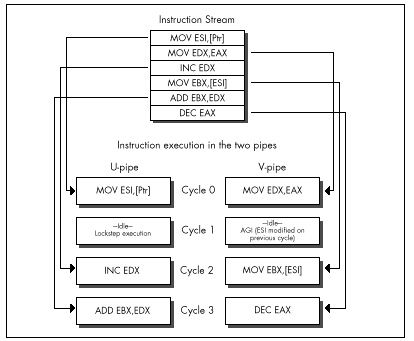
As an example of a sort of AGI that’s new to the Pentium, consider the following test for a NULL pointer, followed by the use of the pointer if it’s not NULL:
push ebx ;U-pipe cycle 1
mov ebx,[Ptr] ;V-pipe cycle 1
and ebx,ebx ;U-pipe cycle 2
jz short IsNull ;V-pipe cycle 2
mov eax,[ebx] ;U-pipe cycle 3 AGI stall
mov edx,[ebp-8] ;V-pipe cycle 3 lockstep idle
;U-pipe cycle 4 mov eax,[ebx]
;V-pipe cycle 4 mov edx,[ebp-8]This commonplace code loses a U-pipe cycle to the AGI caused by
AND EBX,EBX, followed by the attempt two instructions later
to use EBX to point to memory. The code loses a V-pipe cycle as well,
because lockstep execution won’t let the next V-pipe instruction execute
until the paired U-pipe instruction that suffered the AGI finishes. The
solution is to use TEST EBX,EBX instead of
AND; TEST can’t modify EBX, so no AGI occurs. Sure,
AND EBX,EBX doesn’t modify EBX either, but the Pentium
doesn’t know that, so it has to insert the AGI.
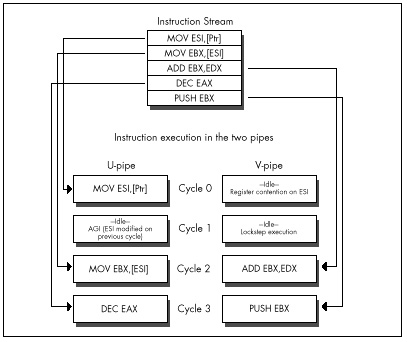
As on the 486, you should keep a careful eye out for AGIs involving
the stack pointer. Implicit modifiers of ESP, such as PUSH
and POP, are special-cased so you don’t have to worry about
AGIs. However, if you explicitly modify ESP with this instruction
sub esp,100hfor example, or with the popular
mov esp,ebpyou can then get AGIs if you attempt to use ESP to address memory, either explicitly with instructions like this one
moveax,[esp+20h]or via PUSH, POP, or other instructions
that implicitly use ESP as an addressing register.
On the 486, any instruction that had both a constant value and an addressing displacement, such as
mov dword ptr [ebp+16],1suffered a 1-cycle penalty, taking a total of 2 cycles. Such
instructions take only one cycle on the Pentium, but they cannot pair,
so they’re still the most expensive sort of MOV. Knowing
this can speed up something as simple as zeroing two memory variables,
as in
sub eax,eax ;U-pipe 1
;any V-pipe pairable
; instruction can go here,
; or SUB could be in V-pipe
mov [MemVar1],eax ;U-pipe 2
mov [MemVar2],eax ;V-pipe 2which should never be slower and should potentially be 0.5 cycles faster, and six bytes smaller than this sequence:
mov [MemVar1],0 ;U-pipe 1
mov [MemVar2],0 ;U-pipe 2Note, however, that my experiments thus far indicate that the two
writes in the first case don’t actually pair (possibly because the
memory variables have never been read into the internal cache), so you
might want to insert an instruction between the two
MOVs—and, of course, this is yet another reason why you
should always measure your code’s actual performance.
Register Contention
Finally, we come to the last major component of superscalar optimization: register contention. The basic premise here is simple: You can’t use the same register in two inherently sequential ways in a single cycle. For example, you can’t execute
inc eax ;U-pipe cycle 1
;V-pipe idle cycle 1
; due to dependency
and ebx,eax ;U-pipe cycle 2in a single cycle; AND EBX,EAX can’t execute until the
value in EAX is known, and that can’t happen until INC EAX
is done. Consequently, the V-pipe idles while INC EAX
executes in the U-pipe. We saw this in the last chapter when we
discussed splitting instructions into simple instructions, and it is by
far the most common sort of register contention, known as
read-after-write register contention. Read-after-write register
contention is the primary reason we have to interleave independent
operations in order to get maximum V-pipe usage.
The other sort of register contention is known as write-after-write. Write-after-write register contention happens when two instructions try to write to the same register on the same cycle. While that may not seem like a particularly useful operation in general, it can happen when subregisters are being set, as in the following
sub eax,eax ;U-pipe cycle 1
;V-pipe idle cycle 1
; due to register contention
mov al,[Var] ;U-pipe cycle 2where an attempt is made to set both EAX and its AL subregister on
the same cycle. Write-after-write contention implies that the two
instructions comprising the above substitute for MOVZX
should have at least one unrelated instruction between them when
SUB EAX,EAX executes in the V-pipe.
Exceptions to Register Contention
Intel has special-cased some very useful exceptions to register contention. Happily, write-after-read operations do not cause contention. Such operations, as in
mov eax,edx ;U-pipe cycle 1
sub edx,edx ;V-pipe cycle 1are free of charge.
Also, stack-related instructions that modify ESP only implicitly
(without ESP as part of any explicit operand) do not cause AGIs, and
neither do they cause register contention with other instructions that
use ESP only implicitly; such instructions include
PUSH *reg/immed*, POP *reg*, and CALL.
(However, these instructions do cause register contention on ESP—but not
AGIs—with instructions that use ESP explicitly, such as
MOV EAX,[ESP+4].) Without this special case, the following
sequence would hardly use the V-pipe at all:
mov eax,[MemVar] ;U-pipe cycle 1
push esi ;V-pipe cycle 1
push eax ;U-pipe cycle 2
push edi ;V-pipe cycle 2
push ebx ;U-pipe cycle 3
call FooTilde ;V-pipe cycle 3But in fact, all the instructions pair, even though ESP is modified five times in the space of six instructions.
The final register-contention special case is both remarkable and remarkably important. There is exactly one sort of instruction that can pair only in the V-pipe: branches. Any near call or conditional or unconditional near jump can execute in the V-pipe paired with any pairable U-pipe instruction, as illustrated by this sequence:
LoopTop:
mov [esi],eax ;U-pipe cycle 1
add esi,4 ;V-pipe cycle 1
dec ecx ;U-pipe cycle 2
jnz LoopTop ;V-pipe cycle 2Branches can’t pair in the U-pipe; a branch that executes in the
U-pipe runs alone, with the V-pipe idle. If a call or jump is correctly
predicted by the Pentium’s branch prediction circuitry (as discussed in
the last chapter), it executes in a single cycle, pairing if it runs in
the V-pipe; if mispredicted, conditional jumps take 4 cycles in the
U-pipe and 5 cycles in the V-pipe, and mispredicted calls and
unconditional jumps take 3 cycles in either pipe. Note that
RET can’t pair.
Who’s in First?
One of the trickiest things about superscalar optimization is that a given instruction stream can execute at a different speed depending on the pipe where it starts execution, because which instruction goes through the U-pipe first determines which of the following instructions will be able to pair. If we take the last example and add one more instruction, the other instructions will go through different pipes than previously, and cause the loop as a whole to take 50 percent longer, even though we only added 25 percent more cycles:
LoopTop:
inc edx ;U-pipe cycle 1
mov [esi],eax ;V-pipe cycle 1
add esi,4 ;U-pipe cycle 2
dec ecx ;V-pipe cycle 2
jnz LoopTop ;U-pipe cycle 3
;V-pipe idle cycle 3
; because JNZ can't
; pair in the U-pipeIt’s actually not hard to figure out which instructions go through
which pipes; just back up until you find an instruction that can’t pair
or can only go through the U-pipe, and work forward from there, given
the knowledge that that instruction executes in the U-pipe. The easiest
thing to look for is branches. All branch target instructions execute in
the U-pipe, as do all instructions after conditional branches that fall
through. Instructions with prefix bytes are generally good U-pipe
markers, although they’re expensive instructions that should be avoided
whenever possible, and have at least one aberration with regard to pipe
usage, as discussed below. Shifts, rotates, ADC, SBB, and
all other instructions not listed in Table 20.1 in the last chapter are
likewise U-pipe markers.
Pentium Optimization in Action
Now, let’s take a look at one of the simplest, tightest pieces of code imaginable, and see what our new Pentium perspective reveals. Listing 21.1 shows a loop implementing the TCP/IP checksum, a 16-bit checksum that wraps carries around to the low bit so that the result is endian-independent. This makes it easy to perform checksums on blocks of data regardless of the endian characteristics of the machines on which those blocks are generated and received. (Thanks to fellow performance enthusiast Terje Mathisen for suggesting this checksum as fertile ground for Pentium optimization, in the ibm.pc/fast.code forum on Bix.) The loop in Listing 21.1 consists of exactly five instructions; it’s hard to imagine that there’s a lot of performance to be wrung from this snippet, right?
LISTING 21.1 L21-1.ASM
; Calculates TCP/IP (16-bit carry-wrapping) checksum for buffer
; starting at ESI, of length ECX words.
; Returns checksum in AX.
; ECX and ESI destroyed.
; All cycle counts assume 32-bit protected mode.
; Assumes buffer length > 0.
; Note that timing indicates that the pipe sequence and
; cycle counts shown (based on documented execution rules)
; differ from the actual execution sequence and cycle counts;
; this loop has been measured to execute in 5 cycles; apparently,
; the 1st half of ADD somehow pairs with the prefix byte, or the
; refix byte gets executed ahead of time.
sub ax,ax ;initialize the checksum
ckloop:
add ax,[esi] ;cycle 1 U-pipe prefix byte
;cycle 1 V-pipe idle (no pairing w/prefix)
;cycle 2 U-pipe 1st half of ADD
;cycle 2 V-pipe idle (register contention)
;cycle 3 U-pipe 2nd half of ADD
;cycle 3 V-pipe idle (register contention)
adc ax,0 ;cycle 4 U-pipe prefix byte
;cycle 4 V-pipe idle (no pairing w/prefix)
;cycle 5 U-pipe ADC AX,0
add esi,2 ;cycle 5 V-pipe
dec ecx ;cycle 6 U-pipe
jnz ckloop ;cycle 6 V-pipeWrong, wrong, wrong! As detailed in Listing 21.1, this loop should
take 6 cycles per checksummed word in 32-bit protected mode, a
ridiculously high number for the Pentium. (You’ll see why I say “should
take,” not “takes,” shortly.) We should lose 2 cycles in each pipe to
the two size prefixes (because the ADDs are 16-bit
operations in a 32-bit segment), and another 2 cycles because of
register contention that arises when ADC AX,0 has to wait
for the result of ADD AX,[ESI]. Then, too, even though
DEC and JNZ can pair and the branch prediction
for JNZ is presumably correct virtually all the time, they
do take a full cycle, and maybe we can do something about that as
well.
The first thing to do is to time the code in Listing 21.1 to verify
our analysis. When I unleashed the Zen timer on Listing 21.1, I found,
to my surprise, that the code actually takes only five cycles per
checksum word processed, not six. A little more experimentation revealed
that adding a size prefix to the two-cycle ADD EAX,[ESI]
instruction doesn’t cost anything, certainly not the one full cycle in
each pipe that a prefix is supposed to take. More experimentation showed
that prefix bytes do cost the documented extra cycle when used with
one-cycle instructions such as MOV. At this point, my
preliminary conclusion is that prefixes can pair with the first cycle of
at least some multiple-cycle instructions. Determining exactly why this
happens will take further research on my part, but the most important
conclusion is that you must measure your code!
The first, obvious thing we can do to Listing 21.1 is change
ADC AX,0 to ADC EAX,0, eliminating a prefix
byte and saving a full cycle. Now we’re down from five to four cycles.
What next?
Listing 21.2 shows one interesting alternative that doesn’t really
buy us anything. Here, we’ve eliminated all size prefixes by doing
byte-sized MOVs and ADDs, but because the size
prefix on ADD AX,[ESI], for whatever reason, didn’t cost
anything in Listing 21.1, our efforts are to no avail—Listing 21.2 still
takes 4 cycles per checksummed word. What’s worth noting about Listing
21.2 is the extent to which the code is broken into simple instructions
and reordered so as to avoid size prefixes, register contention, AGIs,
and data bank conflicts (the latter because both [ESI] and
[ESI+1] are in the same cache data bank, as discussed in
the last chapter).
LISTING 21.2 L21-2.ASM
; Calculates TCP/IP (16-bit carry-wrapping) checksum for buffer
; starting at ESI, of length ECX words.
; Returns checksum in AX.
; High word of EAX, DX, ECX and ESI destroyed.
; All cycle counts assume 32-bit protected mode.
; Assumes buffer length > 0.
sub eax,eax ;initialize the checksum
mov dx,[esi] ;first word to checksum
dec ecx ;we'll do 1 checksum outside the loop
jz short ckloopend ;only 1 checksum to do
add esi,2 ;point to the next word to checksum
ckloop:
add al,dl ;cycle 1 U-pipe
mov dl,[esi] ;cycle 1 V-pipe
adc ah,dh ;cycle 2 U-pipe
mov dh,[esi+1] ;cycle 2 V-pipe
adc eax,0 ;cycle 3 U-pipe
add esi,2 ;cycle 3 V-pipe
dec ecx ;cycle 4 U-pipe
jnz ckloop ;cycle 4 V-pipe
ckloopend:
add ax,dx ;checksum the last word
adc eax,0Listing 21.3 is a more sophisticated attempt to speed up the checksum
calculation. Here we see a hallmark of Pentium optimization: two
operations (the checksumming of the current and next pair of words)
interleaved together to allow both pipes to run at near maximum
capacity. Another hallmark that’s apparent in Listing 21.3 is that
Pentium-optimized code tends to use more registers and require more
instructions than 486-optimized code. Again, note the careful mixing of
byte-sized reads to avoid AGIs, register contention, and cache bank
collisions, in particular the way in which the byte reads of memory are
interspersed with the additions to avoid register contention, and the
placement of ADD ESI,4 to avoid an AGI.
LISTING 21.3 L21-3.ASM
; Calculates TCP/IP (16-bit carry-wrapping) checksum for buffer
; starting at ESI, of length ECX words.
; Returns checksum in AX.
; High word of EAX, BX, EDX, ECX and ESI destroyed.
; All cycle counts assume 32-bit protected mode.
; Assumes buffer length > 0.
sub eax,eax ;initialize the checksum
sub edx,edx ;prepare for later ORing
shr ecx,1 ;we'll do two words per loop
jnc short ckloopsetup ;even number of words
mov ax,[esi] ;do the odd word
jz short ckloopdone ;no more words to checksum
add esi,2 ;point to the next word
ckloopsetup:
mov dx,[esi] ;load most of 1st word to
mov bl,[esi+2] ; checksum (last byte loaded in loop)
dec ecx ;any more dwords to checksum?
jz short ckloopend ;no
ckloop:
mov bh,[esi+3] ;cycle 1 U-pipe
add esi,4 ;cycle 1 V-pipe
shl ebx,16 ;cycle 2 U-pipe
;cycle 2 V-pipe idle
; (register contention)
or ebx,edx ;cycle 3 U-pipe
mov dl,[esi] ;cycle 3 V-pipe
add eax,ebx ;cycle 4 U-pipe
mov bl,[esi+2] ;cycle 4 V-pipe
adc eax,0 ;cycle 5 U-pipe
mov dh,[esi+1] ;cycle 5 V-pipe
dec ecx ;cycle 6 U-pipe
jnz ckloop ;cycle 6 V-pipe
ckloopend:
mov bh,[esi+3] ;checksum the last dword
add ax,dx
adc ax,bx
adc ax,0
mov edx,eax ;compress the 32-bit checksum
shr edx,16 ; into a 16-bit checksum
add ax,dx
adc eax,0
ckloopdone:The checksum loop in Listing 21.3 takes longer than the loop in Listing 21.2, at 6 cycles versus 4 cycles for Listing 21.2—but Listing 21.3 does two checksum operations in those 6 cycles, so we’ve cut the time per checksum addition from 4 to 3 cycles. You might think that this small an improvement doesn’t justify the additional complexity of Listing 21.3, but it is a one-third speedup, well worth it if this is a critical loop—and, in general, if it isn’t critical, there’s no point in hand-tuning it. That’s why I haven’t bothered to try to optimize the non-inner-loop code in Listing 21.3; it’s only executed once per checksum, so it’s unlikely that a cycle or two saved there would make any real-world difference.
Listing 21.3 could be made a bit faster yet with some loop unrolling, but that would make the code quite a bit more complex for relatively little return. Instead, why not make the code more complex and get a big return? Listing 21.4 does exactly that by loading one dword at a time to eliminate both the word prefix of Listing 21.1 and the multiple byte-sized accesses of Listing 21.3. An obvious drawback to this is the considerable complexity needed to ensure that the dword accesses are dword-aligned (remember that unaligned dword accesses cost three cycles each), and to handle buffer lengths that aren’t dword multiples. I’ve handled these problems by requiring that the buffer be dword-aligned and a dword multiple in length, which is of course not always the case in the real world. However, the point of these listings is to illustrate Pentium optimization—dword issues, being non-inner-loop stuff, are solvable details that aren’t germane to the main focus. In any case, the complexity and assumptions are well justified by the performance of this code: three cycles per loop, or 1.5 cycles per checksummed word, more than three times the speed of the original code. Again, note that the actual order in which the instructions are arranged is dictated by the various optimization hazards of the Pentium.
LISTING 21.4 L21-4.ASM
; Calculates TCP/IP (16-bit carry-wrapping) checksum for buffer
; starting at ESI, of length ECX words.
; Returns checksum in AX.
; High word of EAX, ECX, EDX, and ESI destroyed.
; All cycle counts assume 32-bit protected mode.
; Assumes buffer starts on a dword boundary, is a dword multiple
; in length, and length > 0.
sub eax,eax ;initialize the checksum
shr ecx,1 ;we'll do two words per loop
mov edx,[esi] ;preload the first dword
add esi,4 ;point to the next dword
dec ecx ;we'll do 1 checksum outside the loop
jz short ckloopend ;only 1 checksum to do
ckloop:
add eax,edx ;cycle 1 U-pipe
mov edx,[esi] ;cycle 1 V-pipe
adc eax,0 ;cycle 2 U-pipe
add esi,4 ;cycle 2 V-pipe
dec ecx ;cycle 3 U-pipe
jnz ckloop ;cycle 3 V-pipe
ckloopend:
add eax,edx ;checksum the last dword
adc eax,0
mov edx,eax ;compress the 32-bit checksum
shr edx,16 ; into a 16-bit checksum
add ax,dx
adc eax,0Listing 21.5 improves upon Listing 21.4 by processing 2 dwords per loop, thereby bringing the time per checksummed word down to exactly 1 cycle. Listing 21.5 basically does nothing but unroll Listing 21.4’s loop one time, demonstrating that the venerable optimization technique of loop unrolling still has some life left in it on the Pentium. The cost for this is, as usual, increased code size and complexity, and the use of more registers.
LISTING 21.5 L21-5.ASM
; Calculates TCP/IP (16-bit carry-wrapping) checksum for buffer
; starting at ESI, of length ECX words.
; Returns checksum in AX.
; High word of EAX, EBX, ECX, EDX, and ESI destroyed.
; All cycle counts assume 32-bit protected mode.
; Assumes buffer starts on a dword boundary, is a dword multiple
; in length, and length > 0.
sub eax,eax ;initialize the checksum
shr ecx,2 ;we'll do two dwords per loop
jnc short noodddword ;is there an odd dword in buffer?
mov eax,[esi] ;checksum the odd dword
jz short ckloopdone ;no, done
add esi,4 ;point to the next dword
noodddword:
mov edx,[esi] ;preload the first dword
mov ebx,[esi+4] ;preload the second dword
dec ecx ;we'll do 1 checksum outside the loop
jz short ckloopend ;only 1 checksum to do
add esi,8 ;point to the next dword
ckloop:
add eax,edx ;cycle 1 U-pipe
mov edx,[esi] ;cycle 1 V-pipe
adc eax,ebx ;cycle 2 U-pipe
mov ebx,[esi+4] ;cycle 2 V-pipe
adc eax,0 ;cycle 3 U-pipe
add esi,8 ;cycle 3 V-pipe
dec ecx ;cycle 4 U-pipe
jnz ckloop ;cycle 4 V-pipe
ckloopend:
add eax,edx ;checksum the last two dwords
adc eax,ebx
adc eax,0
ckloopdone:
mov edx,eax ;compress the 32-bit checksum
shr edx,16 ; into a 16-bit checksum
add ax,dx
adc eax,0Listing 21.5 is undeniably intricate code, and not the sort of thing one would choose to write as a matter of course. On the other hand, it’s five times as fast as the tight, seemingly-speedy loop in Listing 21.1 (and six times as fast as Listing 21.1 would have been if the prefix byte had behaved as expected). That’s an awful lot of speed to wring out of a five-instruction loop, and the TCP/IP checksum is, in fact, used by network software, an area in which a five-times speedup might make a significant difference in overall system performance.
I don’t claim that Listing 21.5 is the fastest possible way to do a
TCP/IP checksum on a Pentium; in fact, it isn’t. Unrolling the loop one
more time, together with a trick of Terje’s that uses LEA
to advance ESI (neither LEA nor DEC affects
the carry flag, allowing Terje to add the carry from the previous loop
iteration into the next iteration’s checksum via ADC),
produces a version that’s a full 33 percent faster. Nonetheless,
Listings 21.1 through 21.5 illustrate many of the techniques and
considerations in Pentium optimization. Hand-optimization for the
Pentium isn’t simple, and requires careful measurement to check the
efficacy of your optimizations, so reserve it for when you really,
really need it—but when you need it, you need it bad.
A Quick Note on the 386 and 486
I’ve mentioned that Pentium-optimized code does fine on the 486, but not always so well on the 386. On a 486, Listing 21.1 runs at 9 cycles per checksummed word, and Listing 21.5 runs at 2.5 cycles per checksummed word, a healthy 3.6-times speedup. On a 386, Listing 21.1 runs at 22 cycles per word; Listing 21.5 runs at 7 cycles per word, a 3.1-times speedup. As is often the case, Pentium optimization helped the other processors, but not as much as it helped the Pentium, and less on the 386 than on the 486.
Chapter 22 – Zenning and the Flexible Mind
Taking a Spin through What You’ve Learned
And so we come to the end of our journey; for now, at least. What follows is a modest bit of optimization, one which originally served to show readers of Zen of Assembly Language that they had learned more than just bits and pieces of knowledge; that they had also begun to learn how to apply the flexible mind—unconventional, broadly integrative thinking—to approaching high-level optimization at the algorithmic and program design levels. You, of course, need no such reassurance, having just spent 21 chapters learning about the flexible mind in many guises, but I think you’ll find this example instructive nonetheless. Try to stay ahead as the level of optimization rises from instruction elimination to instruction substitution to more creative solutions that involve broader understanding and redesign. We’ll start out by compacting individual instructions and bits of code, but by the end we’ll come up with a solution that involves the very structure of the subroutine, with each instruction carefully integrated into a remarkably compact whole. It’s a neat example of how optimization operates at many levels, some much less determininstic than others—and besides, it’s just plain fun.
Enjoy!
Zenning
In Jeff Duntemann’s excellent book Borland Pascal From Square One (Random House, 1993), there’s a small assembly subroutine that’s designed to be called from a Turbo Pascal program in order to fill the screen or a systemscreen buffer with a specified character/attribute pair in text mode. This subroutine involves only 21 instructions and works perfectly well; however, with what we know, we can compact the subroutine tremendously and speed it up a bit as well. To coin a verb, we can “Zen” this already-tight assembly code to an astonishing degree. In the process, I hope you’ll get a feel for how advanced your assembly skills have become.
Jeff’s original code follows as Listing 22.1 (with some text converted to lowercase in order to match the style of this book), but the comments are mine.
LISTING 22.1 L22-1.ASM
OnStack struc ;data that's stored on the stack after PUSH BP
OldBP dw ? ;caller's BP
RetAddr dw ? ;return address
Filler dw ? ;character to fill the buffer with
Attrib dw ? ;attribute to fill the buffer with
BufSize dw ? ;number of character/attribute pairs to fill
BufOfs dw ? ;buffer offset
BufSeg dw ? ;buffer segment
EndMrk db ? ;marker for the end of the stack frame
OnStack ends
;
ClearS proc near
push bp ;save caller's BP
mov bp,sp ;point to stack frame
cmp word ptr [bp].BufSeg,0 ;skip the fill if a null
jne Start ; pointer is passed
cmp word ptr [bp].BufOfs,0
je Bye
Start: cld ;make STOSW count up
mov ax,[bp].Attrib ;load AX with attribute parameter
and ax,0ff00h ;prepare for merging with fill char
mov bx,[bp].Filler ;load BX with fill char
and bx,0ffh ;prepare for merging with attribute
or ax,bx ;combine attribute and fill char
mov bx,[bp].BufOfs ;load DI with target buffer offset
mov di,bx
mov bx,[bp].BufSeg ;load ES with target buffer segment
mov es,bx
mov cx,[bp].BufSize ;load CX with buffer size
rep stosw ;fill the buffer
Bye: mov sp,bp ;restore original stack pointer
pop bp ; and caller's BP
ret EndMrk-RetAddr-2 ;return, clearing the parms from the stack
ClearS endpThe first thing you’ll notice about Listing 22.1 is that
ClearS uses a REP STOSW instruction. That
means that we’re not going to improve performance by any great amount,
no matter how clever we are. While we can eliminate some cycles, the
bulk of the work in ClearS is done by that one repeated
string instruction, and there’s no way to improve on that.
Does that mean that Listing 22.1 is as good as it can be? Hardly.
While the speed of ClearS is very good, there’s another
side to the optimization equation: size. The whole of
ClearS is 52 bytes long as it stands—but, as we’ll see,
that size is hardly set in stone.
Where do we begin with ClearS? For starters, there’s an
instruction in there that serves no earthly
purpose—MOV SP,BP. SP is guaranteed to be equal to BP at
that point anyway, so why reload it with the same value? Removing that
instruction saves us two bytes.
Well, that was certainly easy enough! We’re not going to find any
more totally non-functional instructions in ClearS,
however, so let’s get on to some serious optimizing. We’ll look first
for cases where we know of better instructions for particular tasks than
those that were chosen. For example, there’s no need to load any
register, whether segment or general, through BX; we can eliminate two
instructions by loading ES and DI directly as shown in Listing 22.2.
LISTING 22.2 L22-2.ASM
ClearS proc near
push bp ;save caller's BP
mov bp,sp ;point to stack frame
cmp word ptr [bp].BufSeg,0 ;skip the fill if a null
jne Start ; pointer is passed
cmp word ptr [bp].BufOfs,0
je Bye
Start: cld ;make STOSW count up
mov ax,[bp].Attrib ;load AX with attribute parameter
and ax,0ff00h ;prepare for merging with fill char
mov bx,[bp].Filler ;load BX with fill char
and bx,0ffh ;prepare for merging with attribute
or ax,bx ;combine attribute and fill char
mov di,[bp].BufOfs ;load DI with target buffer offset
mov es,[bp].BufSeg ;load ES with target buffer segment
mov cx,[bp].BufSize ;load CX with buffer size
rep stosw ;fill the buffer
Bye:
pop bp ;restore caller's BP
ret EndMrk-RetAddr-2 ;return, clearing the parms from the stack
ClearS endp(The OnStack structure definition doesn’t change in any
of our examples, so I’m not going clutter up this chapter by reproducing
it for each new version of ClearS.)
Okay, loading ES and DI directly saves another four bytes. We’ve
squeezed a total of 6 bytes—about 11 percent—out of ClearS.
What next?
Well, LES would serve better than two MOV
instructions for loading ES and DI as shown in Listing 22.3.
LISTING 22.3 L22-3.ASM
ClearS proc near
push bp ;save caller's BP
mov bp,sp ;point to stack frame
cmp word ptr [bp].BufSeg,0 ;skip the fill if a null
jne Start ; pointer is passed
cmp word ptr [bp].BufOfs,0
je Bye
Start: cld ;make STOSW count up
mov ax,[bp].Attrib ;load AX with attribute parameter
and ax,0ff00h ;prepare for merging with fill char
mov bx,[bp].Filler ;load BX with fill char
and bx,0ffh ;prepare for merging with attribute
or ax,bx ;combine attribute and fill char
les di,dword ptr [bp].BufOfs ;load ES:DI with target buffer
;segment:offset
mov cx,[bp].BufSize ;load CX with buffer size
rep stosw ;fill the buffer
Bye:
pop bp ;restore caller's BP
ret EndMrk-RetAddr-2 ;return, clearing the parms from the stack
ClearS endpThat’s good for another three bytes. We’re down to 43 bytes, and counting.
We can save 3 more bytes by clearing the low and high bytes of AX and
BX, respectively, by using SUB *reg8,reg8* rather than
ANDing 16-bit values as shown in Listing 22.4.
LISTING 22.4 L22-4.ASM
ClearS proc near
push bp ;save caller's BP
mov bp,sp ;point to stack frame
cmp word ptr [bp].BufSeg,0 ;skip the fill if a null
jne Start ; pointer is passed
cmp word ptr [bp].BufOfs,0
je Bye
Start: cld ;make STOSW count up
mov ax,[bp].Attrib ;load AX with attribute parameter
sub al,al ;prepare for merging with fill char
mov bx,[bp].Filler ;load BX with fill char
sub bh,bh ;prepare for merging with attribute
or ax,bx ;combine attribute and fill char
les di,dword ptr [bp].BufOfs ;load ES:DI with target buffer
;segment:offset
mov cx,[bp].BufSize ;load CX with buffer size
rep stosw ;fill the buffer
Bye:
pop bp ;restore caller's BP
ret EndMrk-RetAddr-2 ;return, clearing the parms from the stack
ClearS endpNow we’re down to 40 bytes—more than 20 percent smaller than the original code. That’s pretty much it for simple instruction optimizations. Now let’s look for instruction optimizations.
It seems strange to load a word value into AX and then throw away AL. Likewise, it seems strange to load a word value into BX and then throw away BH. However, those steps are necessary because the two modified word values are ORed into a single character/attribute word value that is then used to fill the target buffer.
Let’s step back and see what this code really does, though. All it does in the end is load one byte addressed relative to BP into AH and another byte addressed relative to BP into AL. Heck, we can just do that directly! Presto—we’ve saved another 6 bytes, and turned two word-sized memory accesses into byte-sized memory accesses as well. Listing 22.5 shows the new code.
LISTING 22.5 L22-5.ASM
ClearS proc near
push bp ;save caller's BP
mov bp,sp ;point to stack frame
cmp word ptr [bp].BufSeg,0 ;skip the fill if a null
jne Start ; pointer is passed
cmp word ptr [bp].BufOfs,0
je Bye
Start: cld ;make STOSW count up
mov ah,byte ptr [bp].Attrib[1] ;load AH with attribute
mov al,byte ptr [bp].Filler ;load AL with fill char
les di,dword ptr [bp].BufOfs ;load ES:DI with target buffer segment:offset
mov cx,[bp].BufSize ;load CX with buffer size
rep stosw ;fill the buffer
Bye:
pop bp ;restore caller's BP
ret EndMrk-RetAddr-2 ;return, clearing the parms from the stack
ClearS endp(We could get rid of yet another instruction by having the calling code pack both the attribute and the fill value into the same word, but that’s not part of the specification for this particular routine.)
Another nifty instruction-rearrangement trick saves 6 more bytes.
ClearS checks to see whether the far pointer is null (zero)
at the start of the routine…then loads and uses that same far pointer
later on. Let’s get that pointer into registers and keep it there; that
way we can check to see whether it’s null with a single comparison, and
can use it later without having to reload it from memory. This technique
is shown in Listing 22.6.
LISTING 22.6 L22-6.ASM
ClearS proc near
push bp ;save caller's BP
mov bp,sp ;point to stack frame
les di,dword ptr [bp].BufOfs ;load ES:DI with target buffer;segment:offset
mov ax,es ;put segment where we can test it
or ax,di ;is it a null pointer?
je Bye ;yes, so we're done
Start: cld ;make STOSW count up
mov ah,byte ptr [bp].Attrib[1] ;load AH with attribute
mov al,byte ptr [bp].Filler ;load AL with fill char
mov cx,[bp].BufSize ;load CX with buffer size
rep stosw ;fill the buffer
Bye:
pop bp ;restore caller's BP
ret EndMrk-RetAddr-2 ;return, clearing the parms from the stack
ClearS endpWell. Now we’re down to 28 bytes, having reduced the size of this subroutine by nearly 50 percent. Only 13 instructions remain. Realistically, how much smaller can we make this code?
About one-third smaller yet, as it turns out—but in order to do that,
we must stretch our minds and use the 8088’s instructions in unusual
ways. Let me ask you this: What do most of the instructions in the
current version of ClearS do?
They either load parameters from the stack frame or set up the
registers so that the parameters can be accessed. Mind you, there’s
nothing wrong with the stack-frame-oriented instructions used in
ClearS; those instructions access the stack frame in a
highly efficient way, exactly as the designers of the 8088 intended, and
just as the code generated by a high-level language would. That means
that we aren’t going to be able to improve the code if we don’t bend the
rules a bit.
Let’s think…the parameters are sitting on the stack, and most of our instruction bytes are being used to read bytes off the stack with BP-based addressing…we need a more efficient way to address the stack…the stack…THE STACK!
Ye gods! That’s easy—we can use the stack pointer to address
the stack rather than BP. While it’s true that the stack pointer can’t
be used for mod-reg-rm addressing, as BP can, it can
be used to pop data off the stack—and POP is a one-byte
instruction. Instructions don’t get any shorter than that.
There is one detail to be taken care of before we can put our plan
into action: The return address—the address of the calling code—is on
top of the stack, so the parameters we want can’t be reached with
POP. That’s easily solved, however—we’ll just pop the
return address into an unused register, then branch through that
register when we’re done, as we learned to do in Chapter 14. As we pop
the parameters, we’ll also be removing them from the stack, thereby
neatly avoiding the need to discard them when it’s time to return.
With that problem dealt with, Listing 22.7 shows the Zenned version
of ClearS.
LISTING 22.7 L22-7.ASM
ClearS proc near
pop dx ;get the return address
pop ax ;put fill char into AL
pop bx ;get the attribute
mov ah,bh ;put attribute into AH
pop cx ;get the buffer size
pop di ;get the offset of the buffer origin
pop es ;get the segment of the buffer origin
mov bx,es ;put the segment where we can test it
or bx,di ;null pointer?
je Bye ;yes, so we're done
cld ;make STOSW count up
rep stosw ;do the string store
Bye:
jmp dx ;return to the calling code
ClearS endpAt long last, we’re down to the bare metal. This version of
ClearS is just 19 bytes long. That’s just 37 percent as
long as the original version, without any change whatsoever in the
functionality that ClearS makes available to the calling
code. The code is bound to run a bit faster too, given that there
are far fewer instruction bytes and fewer memory accesses.
All in all, the Zenned version of ClearS is a vast
improvement over the original. Probably not the best possible
implementation—never say never!—but an awfully good one.
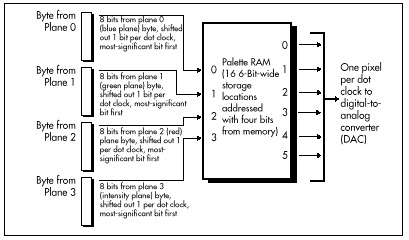
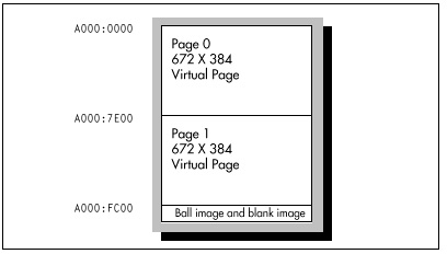
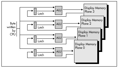
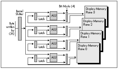
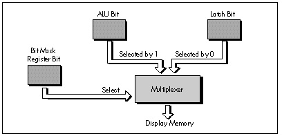
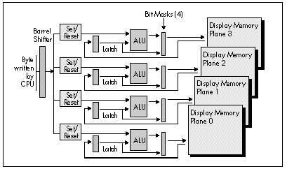
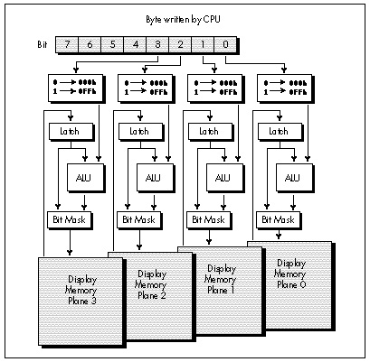
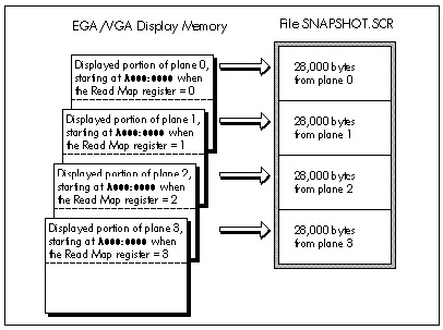
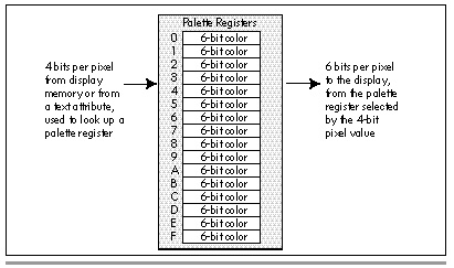
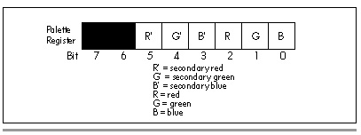
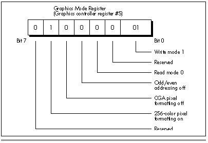
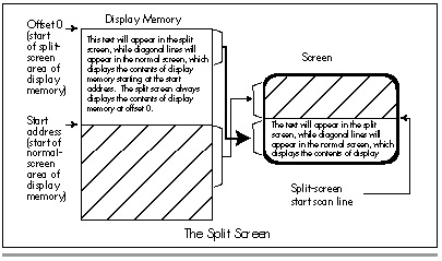
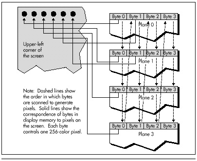
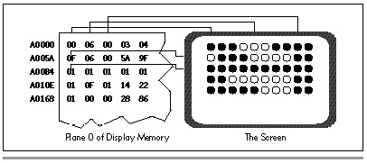
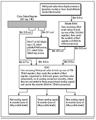
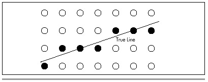
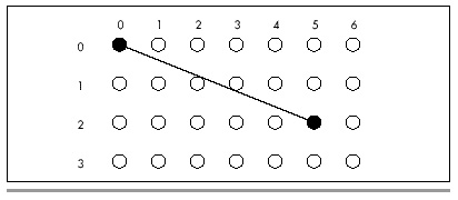
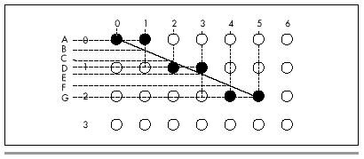
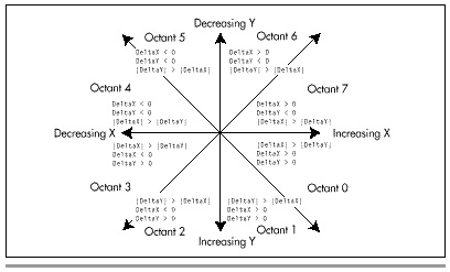
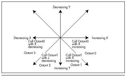
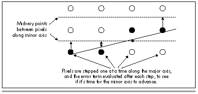
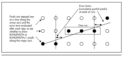
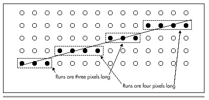
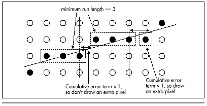
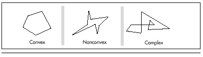
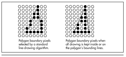
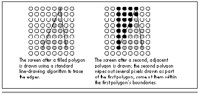
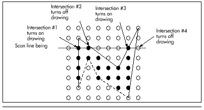
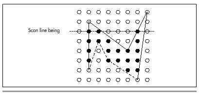
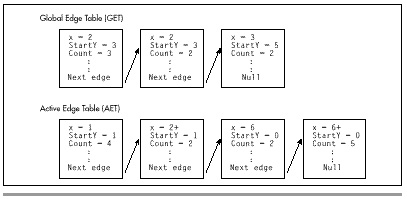
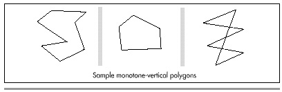
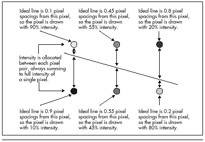

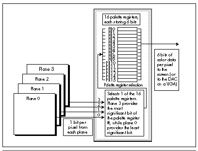
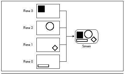
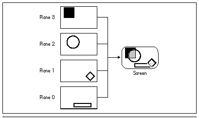
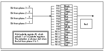
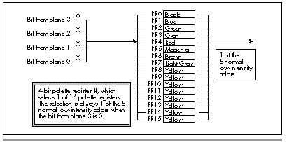
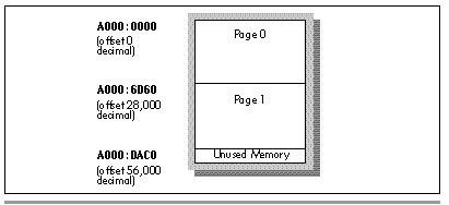
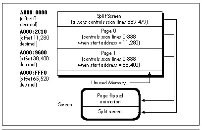
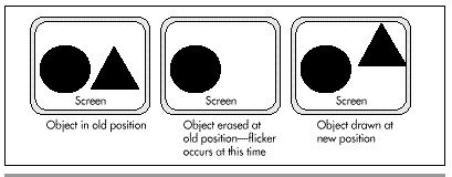
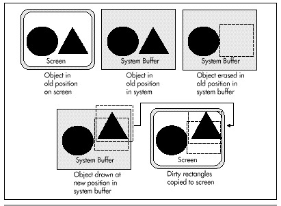
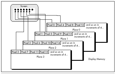
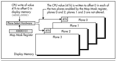
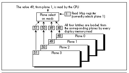
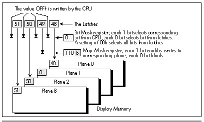
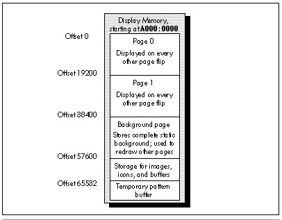
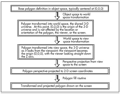
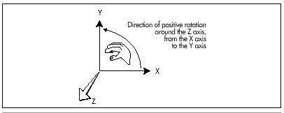
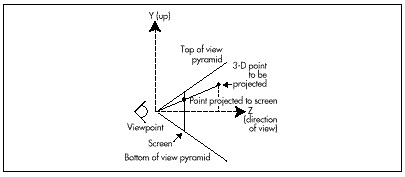
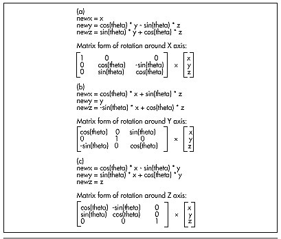
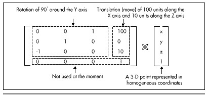
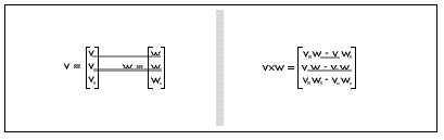
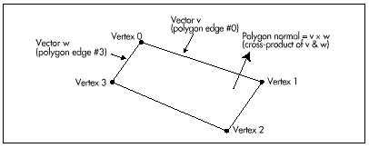
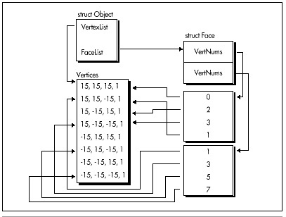
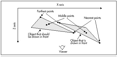
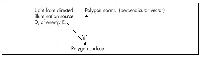
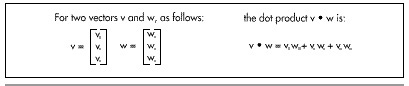
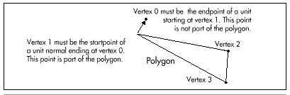
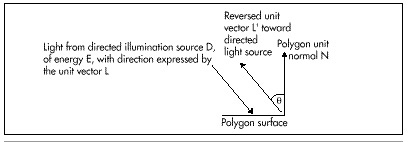
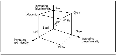
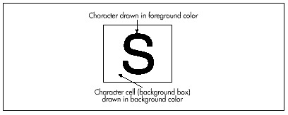
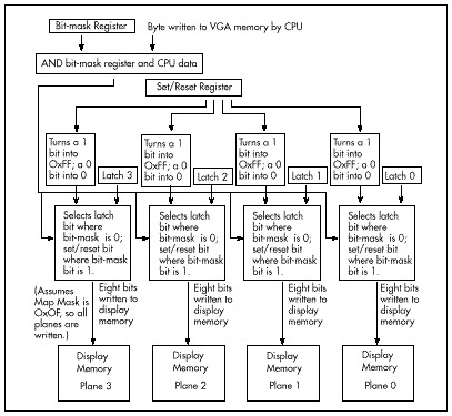
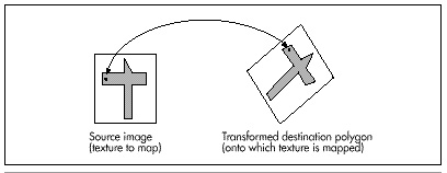
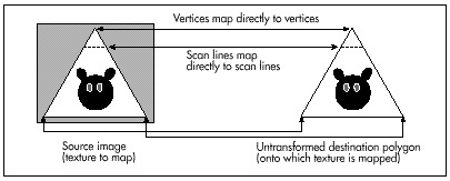
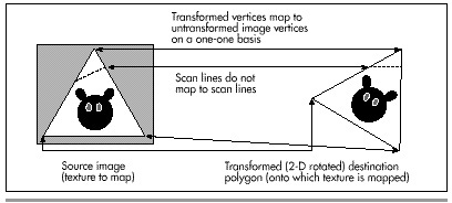
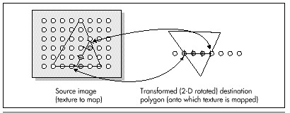
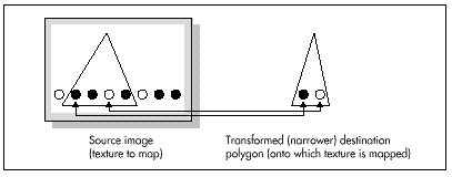
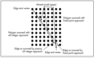
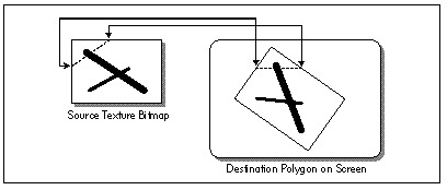
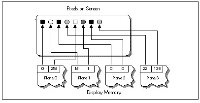
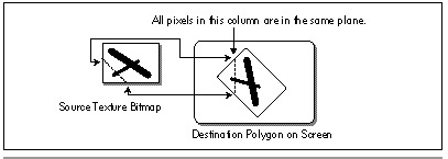
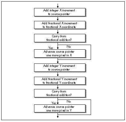
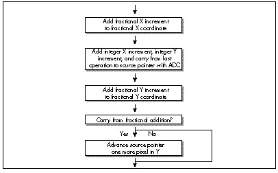
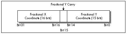
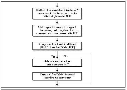
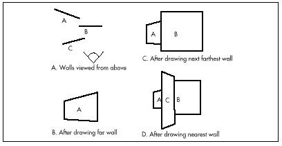
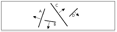
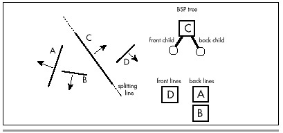
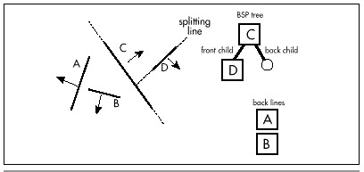
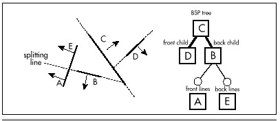
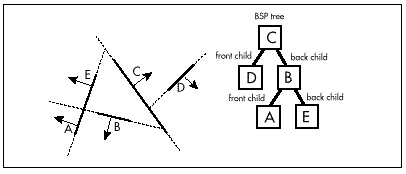
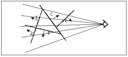
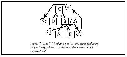
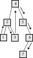
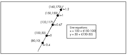
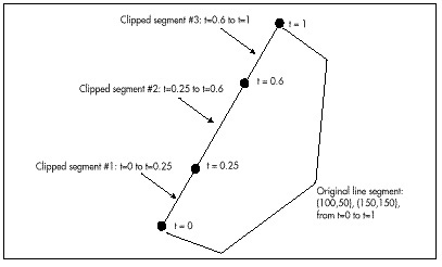
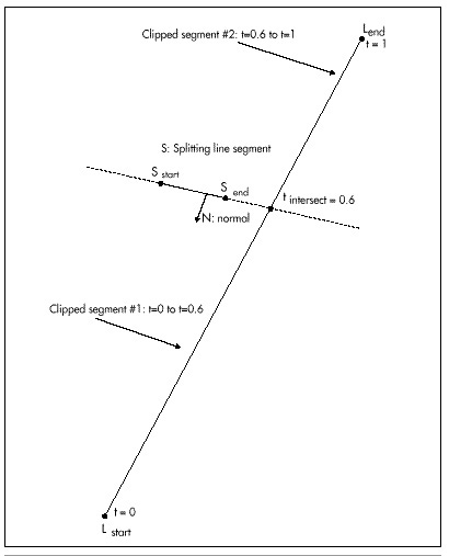
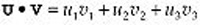

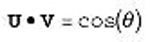
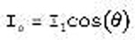
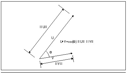
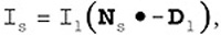
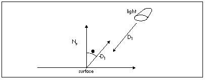
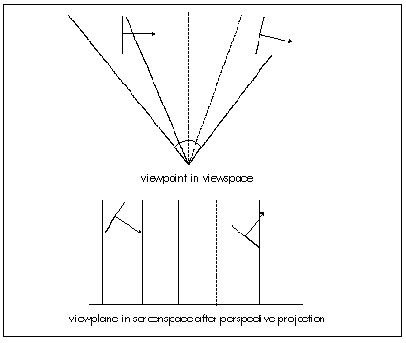

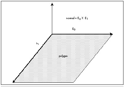
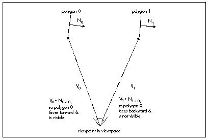

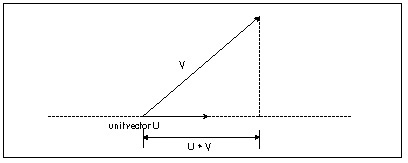
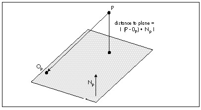
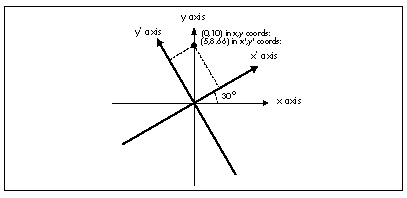
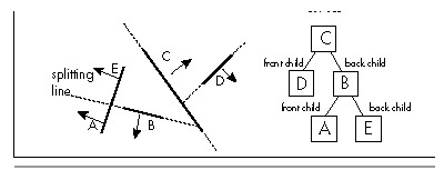
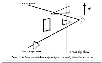
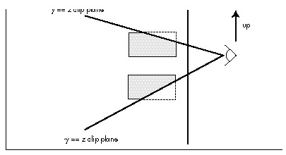
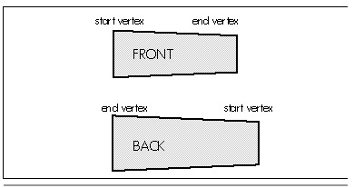
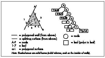
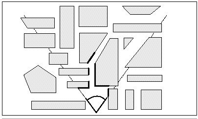
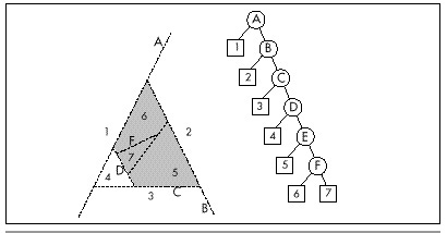
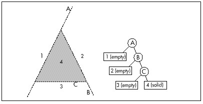
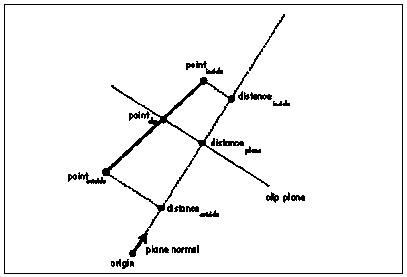
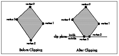
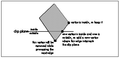
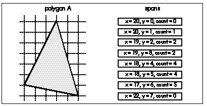
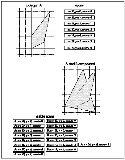
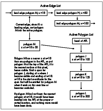
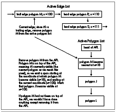
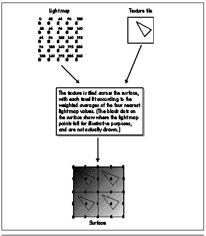
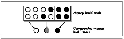
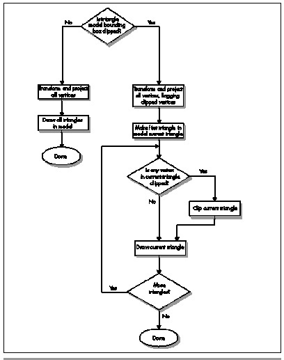
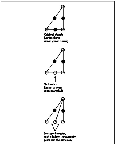
Comments on the C Implementation
EVGALinedoes no error checking whatsoever. My assumption in writingEVGALinewas that it would be ultimately used as the lowest-level primitive of a graphics software package, with operations such as error checking and clipping performed at a higher level. Similarly,EVGALineis tied to the VGA’s screen coordinate system of (0,0) to (639,199) (in mode 0EH), (0,0) to (639,349) (in modes 0FH and 10H), or (0,0) to (639,479) (in mode 12H), with the upper left corner considered to be (0,0). Again, transformation from any coordinate system to the coordinate system used byEVGALinecan be performed at a higher level.EVGALineis specifically designed to do one thing: draw lines into the display memory of the VGA. Additional functionality can be supplied by the code that callsEVGALine.The version of
EVGALineshown in Listing 35.1 is reasonably fast, but it is not as fast as it might be. Inclusion ofEVGADotdirectly intoOctant0andOctant1, and, indeed, inclusion ofOctant0andOctant1directly intoEVGALinewould speed execution by saving the overhead of calling and parameter passing. Handpicked register variables might speed performance as well, as would the use of wordOUTs rather than byteOUTs. A more significant performance increase would come from eliminating separate calculation of the address and mask for each pixel. Since the location of each pixel relative to the previous pixel is known, the address and mask could simply be adjusted from one pixel to the next, rather than recalculated from scratch.These enhancements are not incorporated into the code in Listing 35.1 for a couple of reasons. One reason is that it’s important that the workings of the algorithm be clearly visible in the code, for learning purposes. Once the implementation is understood, rewriting it for improved performance would certainly be a worthwhile exercise. Another reason is that when flat-out speed is needed, assembly language is the best way to go. Why produce hard-to-understand C code to boost speed a bit when assembly-language code can perform the same task at two or more times the speed?
Given which, a high-speed assembly language version of
EVGALinewould seem to be a logical next step.